


Comprehensive information is crucial in process industries. When processing plants operate at optimal range, they increase overall productivity and reduce maintenance costs. Instrumentation assists operators in predicting process problems and planning cost-effective maintenance.
Process measurements can be categorized into point-like and volume measurements. Point-like measurements give process information from a single point in a fixed location, such as temperature, salinity and pH. These measurements often are sufficient for efficient process monitoring and control. However, when operators are working with homogeneities and/or multiple material phases, point-like measurements cannot identify spatial variations.
How a certain material is distributed over a certain volume sometimes becomes more important to effective process monitoring than information from a single point.
Process tomography is a general term for volume measurement techniques intended for cross-sectional or 3-D imaging of material properties and distributions. Tomographic measurements enable noninvasive process monitoring, which can provide valuable information for process optimization and control. The techniques of process monography apply to various industrial positions such as pipes, vessels and reactors.
Electrical Capacitance Tomography
Process tomography covers several tomographic techniques, including electrical, X-ray and ultrasound methods. The imaging technique monitors mixing and sedimentation processes and determines material concentrations in multiphase flows. A specially designed sensor typically carries out the measurements from the target's periphery to avoid disturbing the process.
Process tomography exposes the target to an appropriate stimulus and measures the response. The results depend on the material properties within the target volume.
In X-ray tomography, the target is exposed to X-rays from multiple directions, and the attenuation of intensity is measured along the beam lines. The exposure obtains information on the distribution of the attenuation coefficient.
In electrical tomography, a measurement setup applies excitation signals to the volume. The output signal measurements depend on the electrical properties of the material, such as conductivity or permittivity distribution. A special algorithm estimates the material property distribution.
Electrical capacitance tomography (ECT) is an imaging technique that determines the permittivity distribution of a dielectric medium. Important pioneering work in ECT was carried out at the U.S. Department of Energy, Morgantown Energy Technology Center, U.S., and at the University of Manchester Institute of Science and Technology, U.K.
ECT measurement starts with an ECT sensor. The sensor consists of a set of electrodes mounted around the periphery of the target region. In fixed sensor geometry, the capacitance of each electrode pair depends on the permittivity distribution of the sensor material. The basic procedure for capacitance measurements is to apply an excitation voltage (AC) to one of the electrodes while other electrodes and other physical components are grounded. A potential distribution and an electric field are formed within the sensor, and the underlying permittivity distribution affects the shape of the field. This is because permittivity is a measure of a material's ability to resist external electric fields.
The higher the material permittivity, the weaker the electric field within the material when placed in an external electric field. Figure 1 shows the effect of spatial permittivity changes on the potential distribution. Because of the electric field, electric charges are attracted to the grounded electrodes and are indirectly measured from electric currents. The capacitance data is obtained from the fundamental definition of capacitance C i =Qi/V, where Qiis the charge on the ith electrode and V is the excitation voltage. Each electrode acts as the excitation electrode and the rest as the measurement electrodes, providing a complete set of measurements.
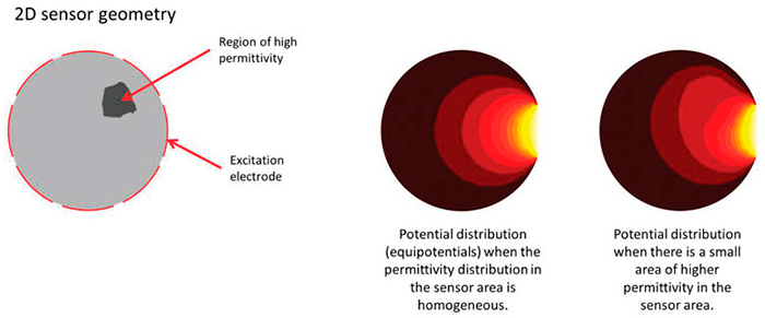 Figure 1. Visualization of the effect of a permittivity inhomogeneity on potential distribution (Images and graphics courtesy of Flowrox Inc.)
Permittivity Distribution Estimates
Capacitance data does not give a clear view on permittivity distribution without experienced professionals interpreting the data. Estimating the permittivity distribution is important for using ECT measurements to their fullest. A realistic mathematical model is needed to simulate capacitance measurements for a given permittivity distribution. Such a model can be derived from the famous Maxwell's equations that form the basis of electromagnetic field theory.
Image reconstruction relies on a permittivity distribution for which the model's predicted observations agree with the actual ECT measurement data. The limited number of capacitance measurements complicates image reconstruction because an infinite number of solutions can produce the same capacitances as the ECT measurements. To reach a stable solution for this problem, additional constraints must be imposed.
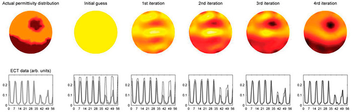 Figure 2. Illustration of the iterative solution of ECT imaging problem. Actual permittivity distribution and measured data are shown in the leftmost panel.
These constraints can be qualitative or quantitative depending on how much is known about the permittivity distribution. Different scaling conditions may require different constraints. ECT imaging begins with an appropriate guess for the permittivity distribution and by gradually proceeding toward model data and measurements (see Figure 2).
ECT is typically used for imaging electrically insulating materials. However, ECT can also be used in cases where the conductivity is not negligible. In such situations, material permittivity is a complex-valued quantity. Solving the real and imaginary parts of the permittivity distribution is essential to the image reconstruction. For this purpose, the measurement system must measure the electrical charges on the electrodes and the phase shift between the charges and excitation voltage.
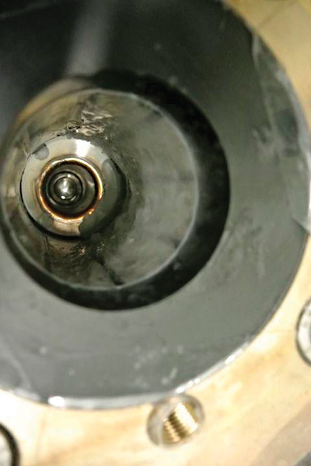 Image 1. Paraffin wax formed on an ECT pipe sensor wall. The thickness of the paraffin layer is about 2 to 3 mm covering four of the eight electrodes.
Detecting Pipeline Scaling
Scaling in pipelines and tanks can be a major problem in process industries. Layers of unwanted substances on equipment surfaces restrict fluid flow, decrease process efficiency or limit heat transfer. Online monitoring of process pipes identifies process scale issues in industries such as chemical, pulp and paper, mining, and wastewater. Having adequate information on the state of scaling in pipelines optimizes cleaning operations, prevents unexpected shutdowns and enhances the effects of anti-scaling chemicals. Depending on the industry, the reduced amount of anti-scaling chemicals can produce significant savings for the user.
Online scaling monitoring systems can use the ECT technique to measure pipe volume and to characterize scale deposits in pipelines. Differences in the electrical properties of the process fluid and unwanted scale materials determine the applicability of ECT measurements. Materials of different electrical properties affect the ECT measurements, and reconstructed ECT images reveal how materials are distributed within the sensor. The estimated permittivity distribution provides information on scaling thickness, scaling growth rate and free volume percentage.
The ECT sensor consists of eight electrodes mounted on the body of the pipeline spool, where they are in contact with process fluid. Some measurement electronics are brought to the sensor, which affects the sensor dimensions. The electrical cabinet contains a power source, a computer for data processing and equipment for remote connections. During installation, a segment of the process pipe is replaced by a sensor with an appropriate inner diameter, and the electrical cabinet is connected to the sensor with a bus cable. After connecting the cabinet to a power source, the system starts and is ready for use.
The scale situation in the sensor can be monitored with a Web-based application, through which measurement settings can be changed. Feedback can also be provided back to the distributed control system (DCS) or control system through a 4-20 mA connection that will provide the amount of pipeline constricted or, conversely, the amount of free pipe available for flow.