More than One Way to Fix a System, Part 2

The various calculations used in the power cost balance sheets in June’s Pump System Improvement column, which were shown in Tables 1 and 2 on page 22 of the June issue of Pumps & Systems (see them below), are documented in industry standards, along with methods covered in fluid dynamics texts. This article will demonstrate these calculations and provide additional details that explain how the conclusions were derived.

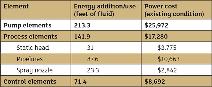Table 1. Power cost balance sheet for the spray system prior to system improvements

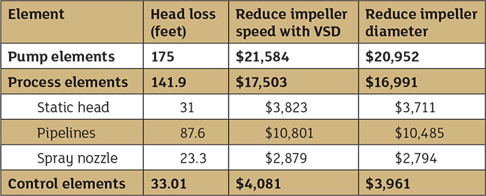Table 2. Comparison costs of reducing impeller speed by incorporating a VSD and reducing impeller diameter

Calculating the Pump Elements

The manufacturer’s supplied pump curve is the primary document for pump operation. A curve for the spray pump is shown here as Figure 2.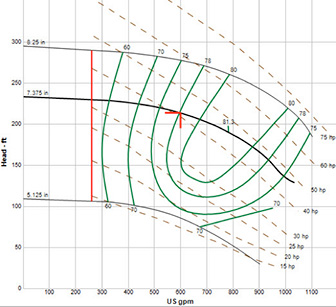

Figure 2. The pump curve for the spray pump operating at 3,550 rpm provides the necessary pump performance data for energy and power calculations. (Graphics provided by the author)

Looking at the curve we can see that the pump with a 7.375-inch impeller operating at 3,550 revolutions per minute (rpm) develops 213.3 feet of head with an efficiency of 78.1 percent. The nameplate on the attached motor shows an efficiency of 94 percent.

With the pump operating 8,000 hours per year and an electrical power cost of $0.10 per kilowatt (kW), the annual operating costs of the spray pump can be calculated using Equation 1.

Inserting the known values into Equation 1 results in the following calculation:

An important point to remember is all the head developed by the pump is consumed by the process and control elements. We will demonstrate how Equation 1 can be used to determine the annual operating cost for each item found in the power cost balance sheet.

Calculating the Process Elements

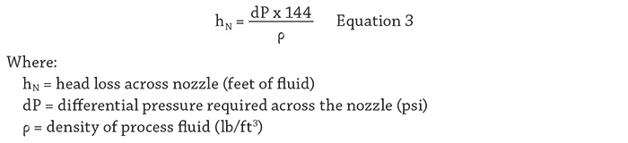
Next, we will look at the process elements using energy to provide the static head across the system; overcome the head loss of the process fluid passing through the pipe, valves and fittings; and provide the differential pressure across the spray nozzle to achieve the proper fluid distribution. All of the system energy is provided by the pump, so if we can determine the head loss across these devices along with the flow rate through them, we can determine the amount of power provided by the pump that is used for each process element item.
We will first look at the energy and power required for the fluid to overcome differences in elevation and pressure across the system.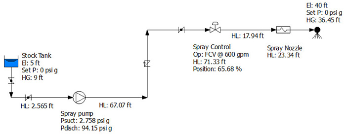

Figure 3. The design data and calculated results needed to perform all head loss and power calculations for the process and control elements

Figure 3 shows that the stock tank is the inlet boundary, and the outlet boundary is the discharge of the spray nozzles into the atmosphere. The static head is calculated using Equation 2.

Inserting the know values into Equation 2 gives us the following calculation:

The spray pump supplies the energy to each item in the system and the static head is only a part of the pump’s total head required, so the annual operating cost can be determined for the static head by using the h_S value calculated in Equation 2 with the head inserted into Equation 1.

Next we will determine the annual operation cost for the system pipelines. The head loss in each pipeline is calculated using the Darcy-Weisbach method found in fluid dynamic texts or Crane Technical Paper 410. The head losses for all pipelines are displayed in Figure 3. The three pipelines are in series, so the head loss for all pipelines in the system can be determined by summing the individual head losses for each pipeline.

The annual operating cost attributed to the pipelines can be determine by using Equation 1 and inserting the pipeline head loss in the equation. This results in an annual operating cost of $10,663 for the pipelines.

The spray nozzle on the spray header was selected by the manufacturer to achieve the user’s desired spray pattern on the moving screen. To meet the user’s needs, the spray nozzle must have a pressure drop of 10 pounds per square inch (psi) across the nozzle. Because the required flow rate is 600 gpm and the density of the process fluid is 61.71 lb/ft³, the head loss across the nozzle is calculated using Equation 3.

Inserting the known values into Equation 3 results in the following:

Inserting this head loss across the spray nozzle into Equation 1 results in an annual operating cost of the spray nozzle of $2,842.

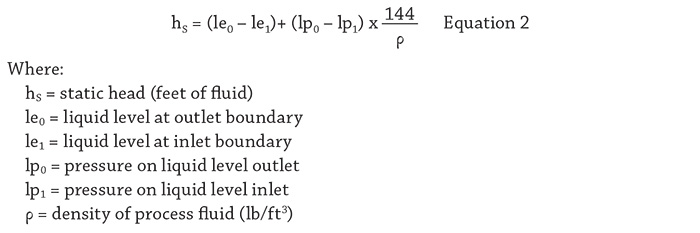
Cost of the Control Valve

The International Society of Automation (ISA) has developed standard ISA-75.01 Flow Equations for Sizing Control Valves, which is used by control valve suppliers for the selection of control valves. The standard consists of a number of equations documenting the process. Control valve selection is outside the scope of this article, but the formulas presented within the standard can be used to determine how a given control valve will operate in the system.

From the plant operating data we know that the flow rate through the spray control valve is 600 gpm, and from the valves stem indicator we can determine the valve position. Using the manufacturer’s supplied control valve data, we can determine the valves C_v, or flow coefficient, for a given valve position. Using the flow coefficient C_v in the valve sizing equations, the differential pressure across the control valve can be calculated. Equation 4 shows the valve sizing equation rearranged to determine the differential pressure.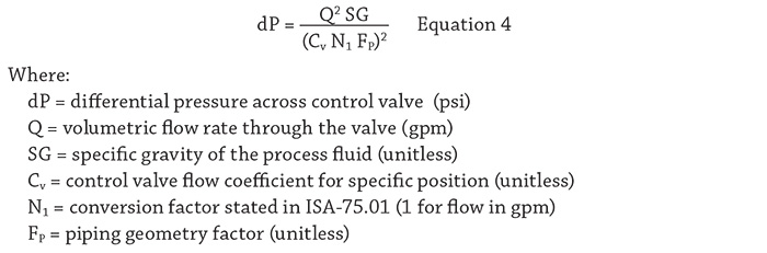

The valve supplier typically includes the piping geometry factor on the valve data sheet for the specific application. The piping geometry factor can also be calculated based on data found in the ISA standard. For this application, the FP equals 0.975. The C_v value through the valve when it is 65.86 percent open is 112.8. Inserting the values into Equation 4 results in:

Converting that differential pressure to head loss results in a value of 71.4 feet if fluid. Using Equation 1 to calculate the annual operating cost of the control elements results in $8,696.

Considering the Options

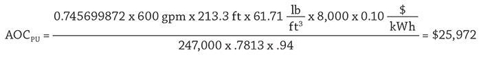
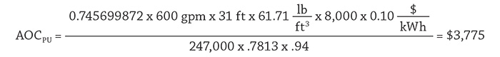
With the power cost balance sheet, we know the pumping cost in operating the system, along with the cost of each item with the system. With this information, we can look for ways to reduce the total cost. In this system, with 71.4 feet of head loss across the control valve and an annual control valve operating cost of $8,696, everyone involved with the system has an estimate on the savings potential.

After discussions with the control valve supplier, we found the spray control will work properly with only a 10 psi pressure drop. Plant staff decided on a 15 psi pressure drop to provide additional operating margin. The control valve equipment supplier was consulted prior to making any plant recommendation. Further, the valve supplier stated that the cavitation occurring within the control valve would be eliminated with a lower differential pressure across the valve.

The pump supplier was asked for ways to reduce differential pressure across the pump by 15 psi. The supplier returned two options: installing a variable speed drive (VSD) to reduce the pump head or reducing the impeller diameter to develop less head.

Saving on operating costs is just one consideration in system improvements, but it helps everyone grasp the magnitude of the possible savings. As a result, a power cost balance sheet was developed for both the VSD option and reducing impeller diameter for system improvement. For each option, we must use the manufacturer’s supplied pump data to arrive at the annual operating cost for the pump elements. Table 3 provides the needed data from the pump curves for each option.

Looking at the variable speed option, installing a VSD reduced the pumping cost to $21,584, while trimming the existing pump impeller results in a pumping cost of $20,952.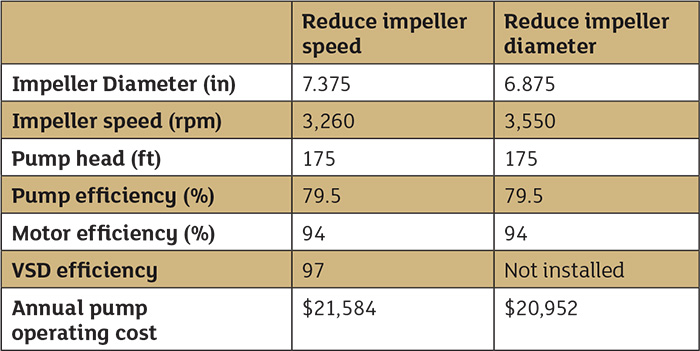

Table 3. The pump performance data for the spray pump with a flow rate of 600 gpm, pumping a fluid with a fluid density of 61.71 lb/ft³

As you can see from Table 3, the pump head produced by both pump options are identical because the objective was to reduce the differential pressure across the control valve to 15 pounds per square inch differential (psid). The reason for the higher operating cost for the VSD option is the addition of the VSD and its associated efficiency of 97 percent, which results in a higher operating cost.

Normally the pump efficiencies of the VSD and the reduced impeller trim options would be different, but in this specific case, the pump efficiency for both options is the same. In looking at Equation 1, the efficiency of the VSD resulted in additional efficiency losses and a higher annual operating cost than the reduced impeller option.

The last thing to point out is that the operation costs of the reduced impeller speed and reduced impeller diameter options are different. The percent of energy used for each item is the same based on the total pump energy. The annual power cost is a function of the efficiency for the various pump elements, so you will notice that the operating cost for each item in the reduced impeller speed option is greater.

Wrapping Things Up

The power cost balance sheet provides detailed cost information for operating existing pumped systems. It provides everyone involved with the project a way to identify the system’s high-cost items and look for ways to make improvements.

The real benefit of the power cost balance sheet is that it allows each improvement option to be calculated and compared with other available options. As shown in this example, a large number of calculations are required to develop this cost data. But with the availability of piping system simulation software and electronic spreadsheets, these tedious calculations can be automated to provide a clear picture of existing costs, along with an accurate estimate on potential cost savings.