Using pump system analysis, from simple to the complex
Multiple pumps operating in complex systems can be synchronized and controlled by a computer. In this column, I will discuss several simplified cases, to give an idea of how pump system interactions are handled and what is involved. This column will also discuss how friction, static, and combination system hydraulics affect the system's results.
Single Pump
First, a simple, single-pump system with friction but no static head portion is shown in Figure 1.
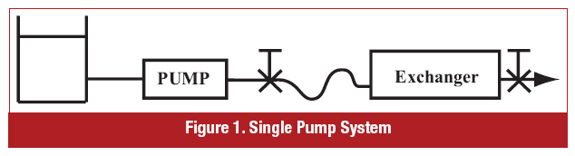
The pump must generate pressure (head) to overcome hydraulic losses in the system. These losses occur in valves, bends, elbows, heat exchanger and pipe friction. Friction head loss is proportional to the square of flow:
HLOSS = K x Q2 (This is an equation of a parabola.)
When:
K = friction coefficient
Q = flow through the system
HLOSS = hydraulic losses through the system
Analogous to an electric circuit, the summation of individual losses is equal to a total system hydraulic loss:
HLOSS = KVALVE x Q2 + KELBOW x Q2 + KHE x Q2 +... =
(KVALVE + KELBOW + KHE +...) x Q2 = KSYSTEM x Q2
The math is easy by adding the individual hydraulic coefficients because the flow is the same throughout the system. We could not do this as easily if the system had branches. This is why it is analogous to the electric circuit, the same current flowing from one component to the next results in different voltage drops across the individual resistors. In hydraulics, the pressure drop due to fluid flow is similar to the voltage drop.
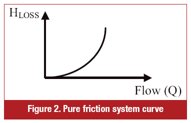
Once the KSYSTEM is calculated, a pure friction (no elevation component) system curve can be plotted. See Figure 2.
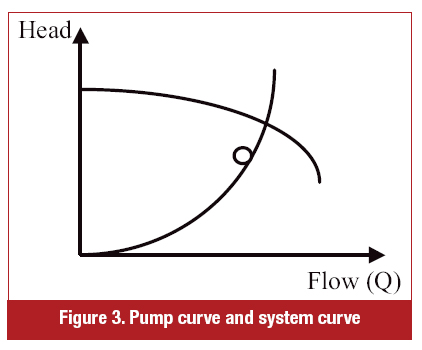
If the pump curve and a system curve are plotted together, an intersection determines the pump's operating point because it belongs to both curves as shown in Figure 3.
Two Pumps in Parallel
Next, we will take a look at two pumps in parallel as shown in Figure 4.
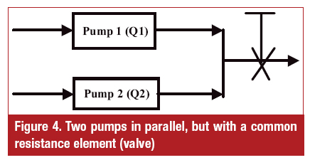
Flows Q1 and Q2 combine, and that is what flows through the valve:
QVALVE = Q1 + Q2
The valve curve is a similar parabola as shown in the previous example:
h = K x QVALVE2 = K x (Q1 + Q2)2
Mathematically, a pump curve is head as a function of flow. It can also be expressed as flow as a function of head, i.e.:
Q1 = f(H1), and Q2 = f(H2)
In general, the pumps do not have to be identical. If they are not identical, then
QTOTAL = Q1+Q2 = f(H1) + f(H2)
Since QTOTAL = QVALVE, the combined pump curve and valve (i.e. system) curves can be plotted, and the intersection determines the head (pressure) where the pump/system will operate as shown in Figure 5.
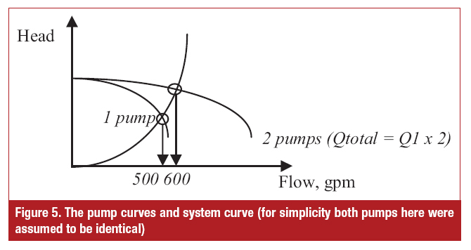
When only one pump was operating, the flow was 500 gallons per minute (gpm). However when the second pump came online, they did not produce twice the flow, (1,000 gpm). Instead, only 600 gpm flows through the system. The reason is the shape of the system's resistance curve. However, if the pumps were pumping against mainly a static head (such as pressurized tank), then the flows would be additive. This is because the static head curve is not a parabola, but a straight line, independent of flow and parallel to the flow axis (Figure 6).
In general, a combination of friction as well as static heads may be present, but one scenario is ususally predominant.
Two Pumps in Parallel with Differing Resistance
In the previous example, the change of the valve setting (changing valve, K, coefficient) affects both pumps the same. However, what if the system is set up as in Figure 7?
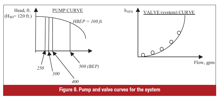
For simplicity, assume that the pumps and valves are identical and that each valve is throttled the same percentage (i.e. having the same coefficient "k"). Several points from the curves have been entered into Table 1.
.jpg)
We know the following:
- There are no other losses except for the valves. In other words, all other losses have been combined into the equivalent valves (V0 and V2).
- Valve V0 sees the combined flows from Pumps 1 and 2.
- The head generated by Pump 1 is equal to the pressure drop (head loss) across V0. Because of the pressure continuity, the nodal point at the exit of Pump 1 is the same as the entry point into V0.
- V2 sees flow from Pump 2 only.
- The system must be in balance to satisfy individual pump H-Q curves and individual valve h-Q curves.
The solution is iterative:
a) Guess at the flow from Pump 1, Q1 = 250 gpm.
b) Per H-Q curve of Pump 1, head H1 = 118 feet.
c) Head loss across valve V0 is equal to the head generated by Pump 1, i.e. valve h1 = H1 = 118 feet.
d) From the V0 curve, Q0 = 543 (We actually "cheated" a bit here—got the equation for the parabola, h0 = Q02/2500—and then just plugged in the numbers).
e) Total pumps flow is equal to what is flowing through V0, i.e. QTOTAL = Q0 = 543.
f) Flow through Pump 2 is the difference: Q2 = Q0 – Q1 = 543-250 = 293 gpm.
g) From the Pump 2 curve (Using identical pumps in this case), H2 = 116 ft. (Approximately, as it is more difficult to derive the polynomial equation for the pumps; for the valve it is easy, a parabola).
h) A pressure drop across V2 is the difference between the pressures at its exit and inlet. The exit pressure is equal to what Pump 1 generated, and the inlet is what Pump 2 generated, i.e. h2 = 116 – 118 = -2 ft.
The solution (-2) is impossible. The first guessed flow from Pump 1 was wrong. Let's try again:
a) New guess, Q1 = 300 gpm
b) H1 = 115 ft.
c) h0 = H1 = 115 ft.
d) Q0 = 536 gpm
e) QTOTAL = Q0 = 536 gpm
f) Q2 = Q0 – Q1 = 536 – 300 = 236 gpm
g) H2 = 119 ft. from pump curve
h) h2 = H2 – H1 = 119 – 115 = 4 ft.
i) From valve curve (or interpolating from the Table), Qvalve2 = 100 gpm
j) Q2 = Qvalve2 = 100 gpm (from the flow continuity – what flows to Valve 2 has to come out of Pump 2).
The solution arrived at above is not equal to Pump 2's flow as derived at Step f. So, we need to guess again. (But we are getting closer).
a) Next guess, Q1 = 400 gpm
b) H1 = 113 ft.
c) h0 = H1 = 113 ft.
d) Q0 = 532 gpm
e) QTOTAL = Q0 = 532 gpm
f) Q2 = Q0 – Q1 = 532-400 = 132 gpm
g) H2 = 119.5 ft. from pump curve
h) h2 = H2 – H1 = 119.5-113 = 6.5 ft.
i) Qvalve2 = 127 gpm
j) Q2 = Qvalve2 = 127 gpm
This solution is a reasonable convergence. Therefore, the final answer is:
Pump 1: flow = 400 gpm, head = 113 ft.
Pump 2: flow = 132 gpm, head = 119.5 ft.
The solution determined above has a numeric (analytical) counterpart and could be solved by writing a set of simultaneous equations and solving them:
H2 = K2 x Q22
H0 = K0 x (Q1+Q2)2 [we could even have different valves or valve settings (different K0 and K2)]
H1 = f(Q1) or Q1 = f(H1)
H2 = f(Q2) or Q2 = f(H2) (pumps also could be different)
H1 = h0
h2 = H1 – H2
In this situation, six equations and six unknowns exist: Q1, Q2, H1, H2, h1, h2.
Clearly, even a simple case of two pumps and two valves can be a time consuming task. For a real pumping system with many pumps and components, a manual method is impractical. This is when computers come handy.
We have only touched on systems with stable curves. What happens if the pump curves are not stable? (See "Pumping Prescriptions," Pumps & Systems, February 2011.) Mathematically, we get multiple solutions. How do programs solve this? That is another issue. For those who might be system solutions enthusiasts, enter the data for Case 3 into a computer program. Let us know if you get a similar answer. If so, a free admission to the next Pump School class is yours. Moreover, you can present your solution to class attendees. (www.pumpingmachinery.com/pump_school/pump_school.htm).
Pumps & Systems, June 2011
Click here to see a Readers Respond to this article.