A phenomenon called water hammer can lead to dangerous scenarios like collapsing pipes and piping getting knocked off its supports. Water hammer occurs when large or small surges in pressure pass quickly through a piping system. Not only does it sound terrible, but it can be incredibly destructive. Water hammer is the process a piping system undergoes as it transitions from one steady-state operation to another. It is present in all piping systems and is not limited to water systems only. A water hammer event can be caused by operational changes that are planned, as well as sudden unplanned upsets.
Sometimes, users claim they do not have water hammer in their system, which is not true. Even when a pump is being started up, water hammer is being introduced into the system. What causes the water hammer event and how bad it can be is what needs to be determined.
The American Society of Mechanical Engineers (ASME) B31.3 and B31.4 piping codes are standards that are broadly applicable to piping systems.1 In ASME B31.3 for process piping, section 301.2.2 discusses required pressure containment or relief. Section 301.2.2 states the following:
a) Provision shall be made to safely contain or relieve any pressure to which the piping may be subjected. Piping
not protected by a pressure relieving device, or that can be isolated from a pressure relieving device, shall be designed for at least the highest pressure that can be developed.
b) Sources of pressure to be considered include ambient influences, pressure oscillations and surges, improper operation, decomposition of unstable fluids, static head and failure of
control devices.
c) The allowances of para. 302.2.4(f) are permitted, provided the other requirements of para. 302.2.4 are
also met.
This requires system designs to account for high pressures. Other sections discuss what occasional pressure variations are and what can be allowed. ASME B31.4 for “Pipeline Transportation Systems for Liquid Hydrocarbons and Other Liquids” also addresses internal design pressures and mentions “pressure rise above maximum stead-state operating pressure due to surges and other variations from normal operations is allowed in accordance with para. 402.2.4.” In section 402.2.4, it states, “Surge calculations shall be made, and adequate controls and protective equipment shall be provided so that the level of pressure rise due to surges and other variations from normal operations shall not exceed the internal design pressure at any point in the piping system and equipment by more than 10%.”
Overall, water hammer and pressure surges must be quantified and addressed to protect the system. Water hammer can be introduced in many ways. The classic example is that of a fast valve closure and is often used to help describe the concepts of water hammer. Water hammer literature covers fast valve closure events quite often as being the most potential disastrous water hammer causes. However, water hammer can also be caused by pump trip events, pump startup events, overpressurization causing relief valves to open and close, control valves failing, check valves slamming, etc.
The classic fast valve closure example often used to describe water hammer will typically discuss the Joukowsky equation, which is used to calculate the maximum theoretical pressure surge for an instantaneous event. The Joukowsky equation depends on the fluid density, wavespeed of the fluid and the change in velocity.2 The Joukowsky equation can be applied to anything that causes an instant change in velocity. Using the Joukowsky equation to determine the maximum theoretical surge pressure is a helpful starting point. However, there are times when it is possible to experience pressure surges larger than the equation predicts.
Example cases where this can happen is if there is transient cavitation present in a system or line packing. That being said, the fast valve closure example is a great way to gain an understanding of water hammer. Various methods are available to quantify the pressure response during a water hammer event, and these calculations can be complicated and strenuous. One method is the Method of Characteristics which solves the transient mass and momentum balance equations in a characteristic grid approach.4 Applying these calculations to a valve closure example to determine how the surge pressure at the valve changes with time is not too difficult. The challenge is that literature often demonstrates a fast valve closure example in the context of a single straight pipe flow path with water and rarely provides guidance or demonstrates calculations for a more complex system with multiple flow paths, pumps, surge suppression devices, etc.
Creating a spreadsheet using the Method of Characteristics to solve for the changing pressures and flow rates in a more complex, multibranched or looped piping system can be done. However, the spreadsheet would be large and impractical. Water hammer analysis software is a useful tool that can aid in conducting a water hammer analysis for simple or complicated systems without requiring a doctoral study in water hammer theory. Water hammer analysis software often takes a one-dimensional approach to solving the system of transient flow rates, pressures, velocities, etc. This can help engineers gain a better understanding to either determine root cause for existing problems or water hammer related accidents, or for preventative approaches to new designs or operational changes.
Consider a water hammer analysis model for the liquefied natural gas (LNG) plant in Image 1. This plant was undergoing an expansion and initially had three pumps operating in parallel. The expansion would bring two additional pumps with a third acting as a spare. Note, there are two sets of pumps with their own riser pipe that tie into a main header. Flow later splits and leads to two separate discharge valves. The pipe runs highlighted with blue are legs where transient force loads are required for pipe stress analysis. The pipe run highlighted in green is a single continuous flow path from pump P-101C to valve LV-1564A2.
There is more to a water hammer analysis than checking the pressure at a closing valve. Transient pressure waves propagate through a piping system at several thousand feet per second and the wave patterns can have interference that can lead to disastrous effects. It is understandable that pipes may rupture at high pressure spikes, but low pressures can be just as problematic. If sub-atmospheric pressures are present, this can cause pipes to collapse. If transient cavitation is happening where the pressure has reached the vapor pressure, large pressure spikes can occur which is like a large balloon popping inside a pipe. This can especially be the case with an LNG facility due to a vapor pressure that is not as low as that of water.
With the task of completing a water hammer analysis for the expansion of this facility, it is important to understand what the water hammer impacts would be on the existing system. One scenario that can be modeled is the classic valve closure example. In Image 1, the two discharge valves at the outlet of the system will be closing within three seconds with a linear valve closure profile. Fast valve closures cause large pressure spikes. A water hammer study can involve several scenarios where valves are closed at different rates to see how fast is too fast and how slow is slow enough. Linear valve closures are often assumed, and typically closing a valve over longer periods of time can help mitigate the water hammer surge pressures seen. However, this is not always the case. Sometimes, with specific types of valves, the change in pressures and flow rates in the system may not be seen until the last few percent of closure. Therefore, closing valves over longer periods of time may not always help.
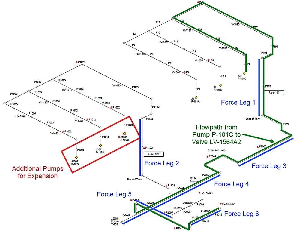
The valve characteristic is also important to consider because how the valve is closed may make a bigger impact on reducing pressure surge than how long the valve is closed. For example, Swaffield & Boldy recommends over a given time of valve closure, if 80% of the valve closure is accomplished in the first 20% of the time it takes to close the valve, and then the remaining 20% of valve closure over the longer 80% of time remaining for the valve closure, the resulting pressure surge can be reduced.5 An example in Image 2 compares two different valve closure rates for an ammonia ship to shore transfer pipeline. The top flow path in Image 2 uses a linear two-second valve closure while the bottom flow path also uses a two-second valve closure but employs the 80/20 closure profile recommended by Swaffield & Boldy.
As seen in Image 2, the 80/20 guideline reduces the transient surge pressure upon valve closure compared to the case with the same closure time with a linear closure profile. This shows the profile in which a valve is closed also makes a difference in water hammer surge pressure reduction as does closing valves over longer periods of time. If not, the profile has more of an impact. Thus, a whole water hammer analysis study can be devoted to determining appropriate valve closure times and profiles which can aid control systems in preventing issues.
Important parameters to evaluate include the minimum and maximum pressures in the system and how they compare to the maximum allowable operation pressure. Other things to evaluate include the possible presence of vapor formation if there is cavitation present in the system, transient performance of components such as how the speed of a pump may change if a pump trip occurs, how the suction and discharge pressure and flow rate may change through a pump during a transient event, how a relief may cycle during a surge situation, etc.
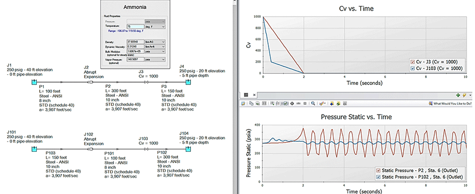
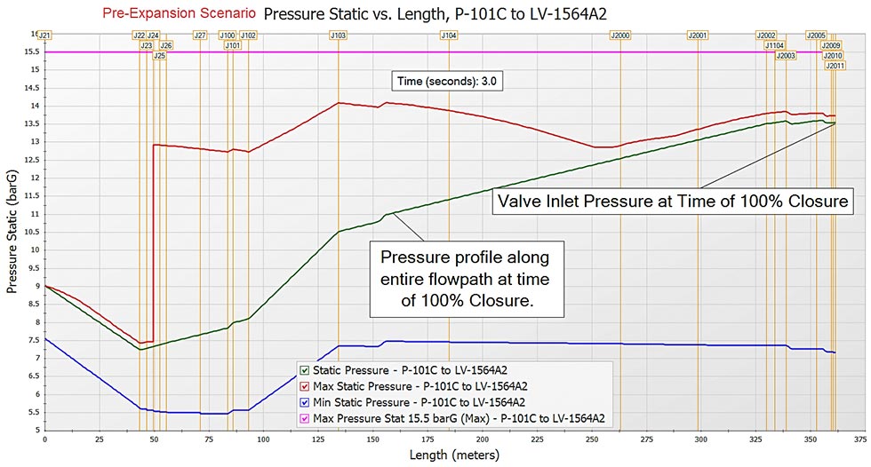
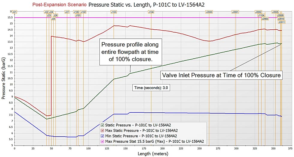
Images 3 and 4 provide the maximum and minimum pressure profile for the flow path highlighted in green from the system in Image 1. Image 3 contains the results for the pre-expansion scenario and Image 3 provides the post-expansion scenario results. In both graphs in Images 3 and 4, the green line in the plot is the pressure along the flow path at the exact time the valves close at three seconds.
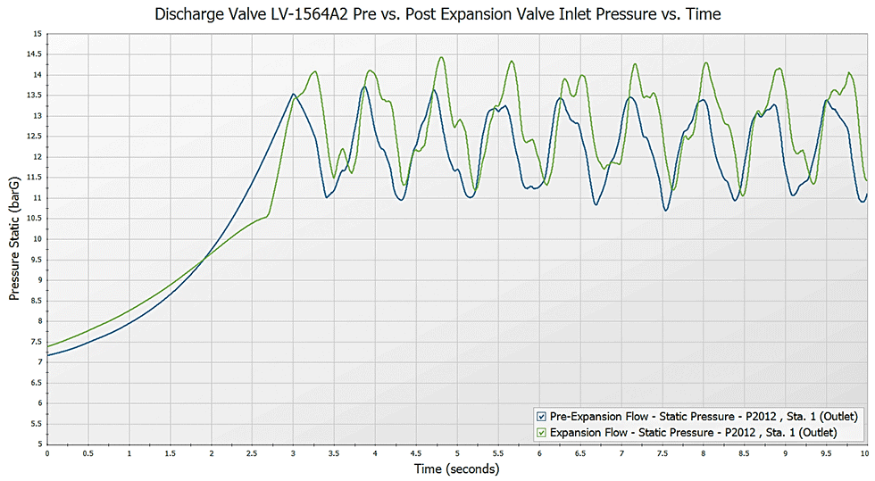
The transient pressure along the flow path at three seconds depicted by the green line in the plots for Images 3 and 4 is similar. Results for the post-expansion scenario with additional pumps operating are similar to the pre-expansion results. Comparing the maximum pressure profiles in Images 3 and 4, the post-expansion scenario does result in higher transient pressures. The reason for this is due to line packing and more flow in the system because the pumps are still operating. This is another example of where the transient pressures can be higher than the prediction of the Joukowsky equation. Image 5 shows more clarity of similar results with the transient pressures at the closing valves inlet over time. Post-expansion pressures at the valve inlet are higher than pre-expansion scenarios but still similar.
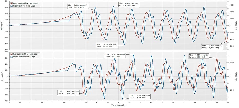
Examining the pipe run force legs in blue (Image 1), the force legs that have the highest transient force loads in both scenarios occur in force legs 3 and 6. The largest force load may occur at the valve that closes, but this is not always the case. There are many hydraulic effects that impact the transient force loads and simply multiplying pressure times area at a location does not provide the correct force values. Water hammer analysis software inherently considers the frictional effects and momentum effects and easily includes these in the force load calculations.6 As shown, it is not easy to assume which force leg the largest transient forces will occur in. Also, the largest forces may not always occur when a valve closes and can happen later in the simulation. This can be due to how the pressure waves interfere with each other in a complex system like in Image 1.
The good news for the LNG plant in Image 1 is the expansion did not result in transient pressures that were higher than the maximum allowable pressure of the system nor did it result in higher transient force loads. The wavespeed in this system is about half of the typical wavespeed. If a different fluid were in this system, the results could be more disastrous and if the system were not carefully analyzed previously, including the force calculations, this could easily uncover a whole new set of issues. In addition, many other scenarios should be evaluated as well such as pump startup scenarios, pump trip scenarios where either all pumps trip together or one pump trips by itself, potentially leading to a large check valve slam event and more.
References
Codes Concerning Water Hammer: ASME B31.3 AND B31.4, waterhammer.com/en/blog/design/codes-concerning-waterhammer-asme-b31-3-and-b31-4
“Water Hammer: What & Why”, pumpsandsystems.com/water-hammer-what-why
“When the Joukowsky Equation Does Not Predict Maximum Water Hammer Pressures”, aft.com/documents/technicalpapers/2019_pvpjournal_when-the-joukowsky-equation-does-not-predict-maximum-water-hammer-pressures.pdf
“Fluid Transients In Systems”, E. Benjamin Wylie & Victor L. Streeter, 1st Edition, 1993
“Pressure Surge in Pipe and Duct Systems”, J.A. Swaffield & Adrian P. Boldy, 1993
“Evaluating Dynamic Loads in Piping Systems Caused by Waterhammer”, J. Wilcox & T. Walters, 2012, aft.com/white-papers/evaluating-dynamic-loads-in-piping-systems-caused-by-waterhammer