This pump setup allows the ability to add or subtract flow capacity.
Grundfos

Many of today’s pumps are installed to operate under variable flow conditions, so understanding the concept of parallel pump control is a must. First, it is critical to know how parallel pumps will operate upon installation.

The idea behind parallel connected pumps is the ability to add or subtract flow capacity and/or provide redundancy. Image 1 shows three parallel connected pumps. For the purpose of this discussion, assume they are each of equal capacity. The pump head-capacity curves are shown in Image 2.

 Three parallel connected pumps and pump head-capacity curves
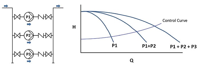
Image 1 (left). Three parallel connected pumps. Image 2 (right). Pump head-capacity curves (Images courtesy of Grundfos)

Shown in these figures is a three-pump setup, often referred to as a “triplex” system, in which flow capacity is added by switching on additional pumps. P1 shows the head-capacity curve for one pump. P1+P2 shows the combined head-capacity for two pumps. P1+P2+P3 shows the combined head-capacity for three pumps. The control curve, which also resembles a system curve at 100 percent design flow, depicts what is required by the piping system in terms of flow and head capacity.

Note that the head required increases as flow increases. Take a closer look at the interaction between the pump head-capacity curves and the control curve.

For years, experts have taught in pump hydraulic courses and articles such as this that pump capacity does not necessarily mean the flow is doubled when two pumps of equal capacity are in operation. This point is often made by describing what is shown in Image 3.

System curve starts at zero flow/zero head and head required in system is constant
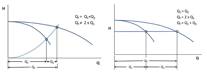
Image 3 (left). System curve starts at zero flow/zero head. Image 4 (right). Head required in system is constant

Image 3 shows a system curve that starts at zero flow/zero head and increases in head with increasing flow. You will notice that the flow capacity added by the second pump (Q2) is not equal to the flow capacity (Q1) provided by the first pump. The system curve shown here is one of pure friction in which there is no static head or fixed control head present in the piping system. It therefore becomes more practical to show a control curve that represents what is actually required in a parallel pumping system.

During the initial part of the parallel pump selection process, little attention is given to the control curve. For example, if a design condition of 800 gallons per minute (gpm) at 100 feet [182 cubic meters per hour (m3/hr) at 30.5 m] is required, the system designer would simply divide the 800 by the number of pumps desired. So, if a two-pump system is desired, each pump would be selected based on 400 gpm at 100 feet (91 m3/hr at 30.5 m).

For purposes of the pump selection process, the flow is doubled when the second pump is added. Upon installation, if the flow of two pumps will exactly double that of one pump, the amount of head required in the system would have to be constant, as shown in Image 4. The control curve in this case would be a straight horizontal line. Actual pump systems that resemble this type of control curve are constant pressure booster systems for high-rise buildings or circulation systems maintaining a constant differential pressure across the pumps.

Realistic control curve and control curve does not intersect head capacity curve for Pump 1N
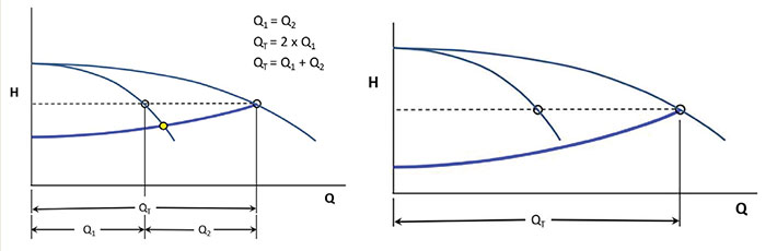
Image 5 (left). Realistic control curve. Image 6 (right). Control curve does not intersect head capacity curve for Pump 1.

A more realistic control curve is shown in Image 5. You will notice that the control curve intersects the head-capacity curve of the first pump at a flow slightly above half of the total design flow, QT. This control curve is representative of how most variable flow pumping systems are configured to operate. A key takeaway from this figure is that the control curve intersects both pump head-capacity curves. Once parallel pumps have been selected, ensuring the control curve intersects all connected pumps will help prevent control challenges once the pumps have been put into operation.

What if the control curve does not intersect one or all of the pump head-capacity curves? Image 6 demonstrates this common scenario. Notice that the control curve does not intersect the head-capacity curve for the first pump. Back in the days of fixed speed pumps, this was a real challenge and typically resulted in some kind equipment change, either pump modification or a valve adjustment of some kind. But in today’s world of variable speed pumping, this type of situation is less of a challenge and can be solved without an equipment modification in most cases. The solution can come in the form of software or pump control logic.

When variable speed drives are to be used for pump control, the total possible operating range can be shown with Image 7. The darker shaded area of the full operational range for pump 1 and the lighter shaded area is the combined operational range for both pumps 1 and 2.

Operating range when variable speed drives are used for pump control
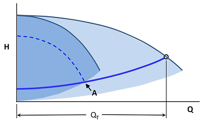
Image 7. Operating range when variable speed drives are used for pump control

So far, we have been looking at the pump head-capacity curves at full speed, or nominal motor speed. The dashed line in Image 7 represents the pump performance at a reduced speed, such as 80 percent. To maintain the required system control head, the second pump must be started at or before this speed. Once the control curve exits the operational area (dark shade) of the first pump, the second pump must be in operation. This can be accomplished in many ways in terms of pump sequencing. Point A on the curve represents where the system control curve exits the operational area of the first pump. We know a few pieces of information about this point: pump speed, pump flow and pump head.

Two practical ways to set up sequencing in this case would be speed or flow. Speed is the least expensive method, as this information can be taken directly from the variable frequency drive (VFD) to the control unit. Flow can either be measured with a flow sensor or calculated based on pump information contained in the drive controls.

Another sequencing method that can be effective in this case would be efficiency-based staging. Since the pump efficiency at the end of the curve is usually low, the second pump would be staged on well before the pump reached 80 percent speed.