Specific speed is a concept developed for water turbines in 1915, which was later applied to centrifugal pumps (Stepanoff, 1948). Specific speed is a way to “normalize” the performance of these hydraulic machines.
The commonly-used equation for specific speed is as follows:
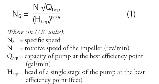
When I was first introduced to specific speed, I must admit to being unimpressed. It appeared to me that the concept might be useful to pump designers, but I could see no value to the end user. I later learned that the concept is essential to the designer, and—because it indicates the shape of the head, power and efficiency curves and the maximum achievable efficiency—it is also of value to end users.
One of the definitions of specific speed is that it is the speed that a modeled pump would run to produce a one foot head when pumping one gallon per minute, but I find that definition awkward.
I prefer to think of it as an index number. In Europe, specific speed is sometimes called the “shape number,” and I prefer that name. It indicates the shapes of the performance curves and also determines, to a large degree, the profile shape of the impeller.
An impeller with a low specific speed has a thin profile (the shrouds are close together) and a large outside diameter (OD) relative to the eye diameter. An impeller with a high specific speed has a fat profile (the shrouds are far apart) and has an eye diameter that is closer in size to the impeller OD.
Figure 1 helps illustrate the concept. The chart was developed years ago by the Worthington Group and is used extensively by the industry. Note that the values of specific speed, in U.S. units, are tabulated along the bottom of the graph. The small drawings below the graph show the profiles of the impellers that correspond to the specific speed numbers.
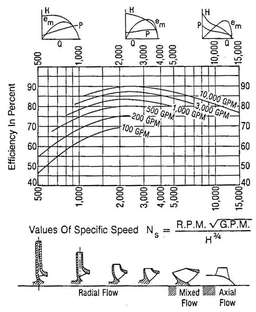
Figure 1
The small performance curves across the top of the graph illustrate the typical shapes of the performance curves correspondent to the values of specific speed. Note that pumps with a low specific speed have a flat head curve, sometimes with a slight droop at shut-off (zero capacity). Such a droop does not make the pump unstable. The power curve is steep. It increases significantly from shut-off to best efficiency point (BEP).
In the midrange of NS values, the head curve continually rises to shut-off, and the power curve changes little from shut-off to BEP. When NS exceeds about 5,000, the slope of the power curve reverses, with the maximum value being at shut-off, and the head curve is very steep, with the shut-off value being as much as three times the BEP value. (Don't start one of these guys with the discharge valve closed.)
Derivation
For those who wish to see a derivation of NS, the following is offered. I use what is called the “modeling law” or “model law” or “factoring law.” This “law” is used when a designer wishes to “model” a pump to one of a different size.
Each dimension of the pump is multiplied by the same factor, the modeling factor, “f.” The existing pump is designated with the subscript “1” and the new pump with the subscript “2.” Then:
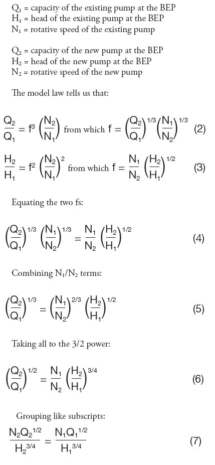
The resultant is specific speed. When one pump is modeled from another, both pumps have the same specific speed.
Making It Unitless
It is commonly said that specific speed is unitless, but it normally is not. In the U.S., with the above units, it is not unitless. It can be made unitless, though, by converting the speed to radians/second, the capacity to cubic feet/second and by multiplying the head by the gravitational constant “g.”
The NS values on the Worthington graph run from 500 to 15,000. What would the values be if we were to convert to unitless numbers? We must divide N by 9.55 to convert to radians/second. Q must be divided by 449 to convert to ft3/second and H must be multiplied by 32.2.
The result tells us that to convert from U.S. units to dimensionless values requires that the U.S. values for NS be divided by 2,735. Therefore, the 500 would become about 1/5, the 15,000 would become about 5, and the unitless value of 1.0 would fall very near the center of the graph, where maximum efficiencies reach their peak.
Is there any significance to the maximum efficiencies occurring where the unitless NS is 1.0? I don't know, but it sure seems like a happy coincidence.
References
- Stepanoff, A. J., Centrifugal and Axial Flow Pumps, John Wiley & Sons, New York, 1948.
- Stepanoff, A. J., Pumps and Blowers – Two-Phase Flow, John Wiley & Sons, New York, 1965.
Notes
- A reaction turbine is, basically, just a centrifugal pump running backwards, with the fluid being pushed backwards through it.
- If it's a double-suction impeller, do not divide by 2. With suction specific speed, we divide the capacity by 2, but not for (discharge) specific speed.
Pumps & Systems, September 2011