Pump system optimization starts with one thing: demand. The engineering marvels that are designed and built must meet a demand to be useful to people. Car engines need to meet power demands so people can drive. Skyscrapers need to meet expected capacity demand to be suitable for business and residential usage. Pipelines and piping are no different. For the industry, the demand typically simplifies to a supplied flow rate, pressure or temperature. Water municipalities need to supply an available flow rate for their constituents. Oil pipelines need a specified pressure to transport crude oil to refineries and ship loading sites. Chemical processes often demand a specific temperature range in order to produce a wide variety of chemical goods. To optimize pumps and systems, it is important to first understand demand and how a pump system can meet it.
As one half of the tag duo, the pump is what produces the flow and pressure to achieve the demand. The pump system operating point is where the pump curve and system curve intersect. This is because the head required by the system for a particular flow rate (demand) is produced by the pump for that same flow rate. The two are in equilibrium. Image 1 demonstrates a standard pump and system curve graph illustrating this equilibrium. The operating point is the intersection of the two curves around 300 gallons per minute (gpm) and 40 feet of head.
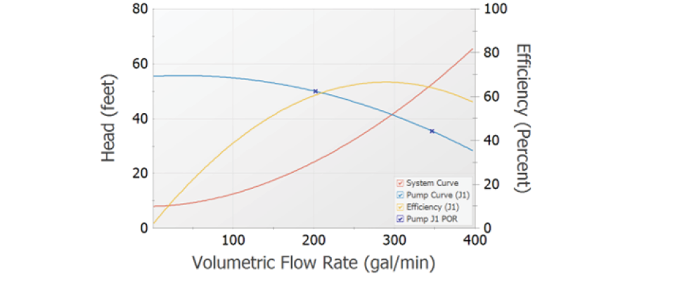
The best efficiency point (BEP) of a pump is key to understanding a pump’s performance. The BEP is where the pump manufacturer designed their pump to operate. This is because it is the point where the pump is most efficient. Think about this idea of inefficiency. The power required from the motor to rotate the pump impeller does not get perfectly transferred into the fluid to propel it, though the goal is for it to transfer as much of it as possible. The additional energy not being transferred into the fluid must go somewhere, typically in the form of heat, sound, vibrations and recirculation. All these inefficiencies are poised to destroy the pump, either through damaging seals, bearings or other wearable components. The best way to mitigate this is to operate near the BEP. American National Standards Institute (ANSI)/Hydraulic Institute (HI) Standard 9.6.3 states that pumps should operate between 70% and 120% of the BEP flow rate to improve energy usage and reliability.
Another valuable reason to operate at the BEP is that the more efficiently energy is transferred to the fluid for transportation, the less energy needs to be expended. Electricity expended by the pump can be a significant bill that adds up over the years and can soon rival the cost of the piping infrastructure. The power required by the pump can be defined by the following equation relating to a fluid’s flow rate, density, gravity, head produced by the pump and the pump’s efficiency:
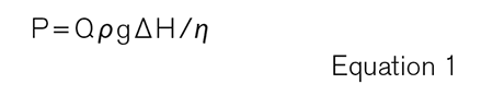
If the flow rate demand and the density of the fluid being worked with are set and gravity is a global constant, there are two ways the power required can be lowered: by operating the pump at a higher efficiency and/or by lowering the head required by the pump. Operating at a higher efficiency is done by running near the BEP. Lowering the head required by the pump is achieved by focusing on the second half of the optimization: the system.
The system is what is resisting the fluid flow. The higher the resistance in the system, the greater the pressure required to push the fluid through the system. What impacts the head required by a flow path in piping and pipelines? Consider the following equation:
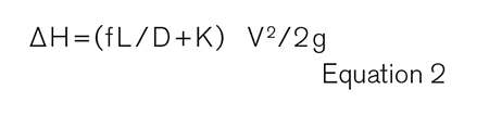
Perhaps the pipe length can be shortened? This is unlikely, as an optimal path has likely already been picked or there are space limitations. What about increasing the diameter or lowering the velocity? Usually, these two are done in tandem because if the flow rate is fixed, increasing the diameter will lower the velocity. This indicates that a larger pipe will require less power from the pump. However, there is a diminishing return. All pipes cannot be 72 inches just because it will require the least amount of power for the flow rate. Pipes are expensive, and that is not even considering that the pump would also be expensive and not operating around its BEP. All projects are unique, but one estimate for a pipe’s cost for materials and installation is $250,000 per inch-mile.
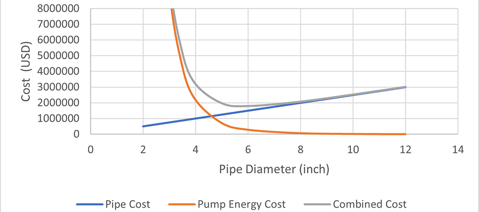
To determine the most economical pipe diameter, the cost of energy to operate the pump and the cost of the piping can be determined for a range of pipe diameters. Note Image 2 as an example. For a set flow rate to meet demand, the smaller the pipe, the cheaper it is to procure. However, the trade-off is the pump would need to push the flow at a higher velocity. The higher the velocity, the more resistance the fluid experiences in the pipe. The higher the resistance, the more power the pump needs to supply. Depending on the expected life of the pump system, a balance between the two costs can be found. Within the graph, the savings of selecting a 6-inch pipe over a 4-inch pipe could be a 50% reduction in power consumption over its estimated 60-year lifespan.
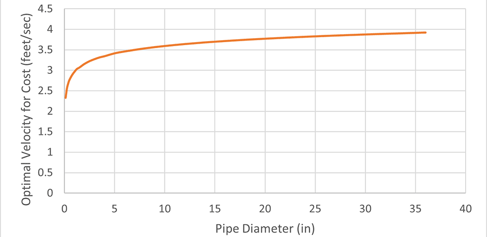
If the flow rate is set, changing the diameter changes the velocity. This can be expanded to show that there is an optimal flow velocity to aim for in piping systems. Taking the previous idea about having an optimal pipe size (and thus optimal flow velocity for a set flow rate), velocity and pipe diameter can be linked together. An optimal velocity for the lowest combined cost of piping and pump energy is often between 3 and 4 feet per second with a pump running at 70% efficiency, with steel piping and operating for 60 years. This confirms a rule of thumb for the water industry, which aims for 3 to 5 feet per second flow velocity.
The graphs in Image 2 and Image 3 are conceptual examples with rough numbers. For a real-world system, analysis should still be done to find these optimal pipe sizes and velocities to meet the demand. However, the overall concepts will remain the same. A larger pipe size, while more expensive upfront, may be more economical over the lifetime of the pump system, and selecting a modest velocity goes a long way for an optimal design.
Running a pump around BEP and selecting the right pipe size before installation are not the only ways to optimize a system. Often, the system is already created, and an employer is not going to take swapping a pump or replacing huge lengths of pipe lightly. Those pieces of equipment are expensive, after all. An option in that case is for a variable speed drive (VSD) to be installed on an existing pump. This allows for more control of the pump by lowering the pump curve to the demand set point and getting closer to the BEP. It is estimated that using a VSD could save as much as 30% of the pump’s energy required to meet a demand that normally would have been expended by a regular control valve throttling the flow.