The peak efficiency achieved in the design point of pumps of different specific speeds1 has not changed much in the past few decades. It seems that most commercially available (and engineered) machines approach an invisible efficiency limit: the empirical values of optimal efficiency can be exceeded only by 1% to 3% with the help of modern automated geometric optimization methods. As a rough estimate, a medium to large size pump has a peak efficiency of about 70% to 90%.2 Considering the complete hydraulic system, however, the average system efficiency is less than about 40%.3
Selecting the pump that best fits a given hydraulic system and the control methods of the pump systems offer large energy savings. Pumps consume between 20 to 60% of the total electricity usage of many industrial, water and wastewater facilities.4 The energy saving opportunity has an impact on the profitability of the named industries, and it is also important in reducing carbon dioxide (CO2) emissions. Thus, energy optimization can contribute to achieving a carbon-free world.
Every megawatt-hour (MWh) of electric energy saved can reduce the CO2 emission by about 0.6 metric tons. The full potential of energy saving can be achieved only by system level modeling and optimization of hydraulic and thermal processes and their control scheme while respecting operational constraints. Detailed guidelines are published in the Hydraulic Institute guide for improved energy efficiency, reliability and profitability.2
The energetic revision of pump systems is an optimization task; the objective function of which can be given either in the form of the life cycle cost (LCC) calculated by the remaining life of the system or by the payback time of the conversion.
The modified system must also cover rare operating conditions, such as startup and future operating modes. It may be necessary to consider additional side conditions, such as prescribed pressure limits or the suction capacity of the pumps.
The topology of the system is described as a general looped network, based on which, the equilibrium thermo-hydraulic state is calculated with Kirchhoff’s laws using Newton-Raphson iteration.5 Dosing and transport of drag-reducing agents (DRA) can be considered in terms of pipe friction factors and material costs. The method allows a quick evaluation of the equilibrium state based on the specified technological conditions (e.g., prescribed pressures or volume flows), design parameters (e.g., pipe length, pipe diameter, pump impeller diameter) and control parameters (e.g., valve settings, pump speed).
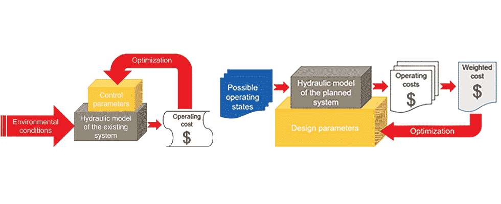
For a relatively simple network with a few loops, up to hundreds of states per second can be evaluated along with the associated cost. The cost function can depend on the system state indicators in general. Optimizing system design parameters is a more complex task than optimizing control parameters, as the designer must consider various operating conditions with different durations. The difference between these two tasks is illustrated in Image 1.
A typical example of control optimization is the control of a power plant condenser cooling system. The number of pumps in operation, the inlet guide-vane angle of the pumps, the position of the throttle valve of the condensers and the condition of the hot water recirculation gates must be determined so that the power plant is operating in the most economical condition.
The cost calculation should consider the dependence of electric output power on the cooling conditions, the pumping cost and the cooling water utilization fee.
Optimization can, in principle, be performed in a discrete parameter space of any number of dimensions, by the stochastic, population-based particle-swarm method,6 using orthogonal sampling for initialization and optional swarm redistribution heuristics if convergence slows down, or—in the case of relatively small-size problems—by simple search based on factorial design. The advantage of this method is that it allows the optimization of discontinuous parameters, such as valve opening-closing or even the type of pumps and other components (component selection).
The quality of the optimum depends on the accuracy of the model describing the behavior of the thermo-hydraulic system. The component characteristics are subject to uncertainties due to design approximations, manufacturing inaccuracies, wear and contamination during operation. The model accuracy can be improved based on diagnostic measurements or data extracted from the automation system. Tuning the uncertain model parameters is also an optimization task: the deviation of model predictions from the measurement data needs to be minimized.
The physics-based modeling approach supplemented with data driven automatic calibration provides means to observe not-measured system parameters or improve parameter values that have a high measurement uncertainty. The detailed system simulation data helps to pinpoint suboptimal system configuration, and, with the help of the optimizer, the component selection process can be sped up. This process can be further aided with the continuously developed element library for typical energy management use cases.
Energy and cost savings can also be achieved through the optimal operation of oil pipelines. Pipelines can typically transport from a single starting point to multiple users. In the case of crude oil pipelines, the starting point is usually an oil field or a port from which the crude oil is delivered to several refineries. Petrol product pipelines transport from the refinery to the logistics centers. The operator delivers the specified fluid masses to the specified destinations within a given time frame. Both the starting pumping station and any additional booster pumping stations, along the pipeline, may contain several different pumps, among which variable frequency drive (VFD)-controlled machines are found. In the case of crude oil pipelines, the dosing of DRA can increase the intensity of transport, but the cost of DRA may exceed the operating cost of the pumps.7
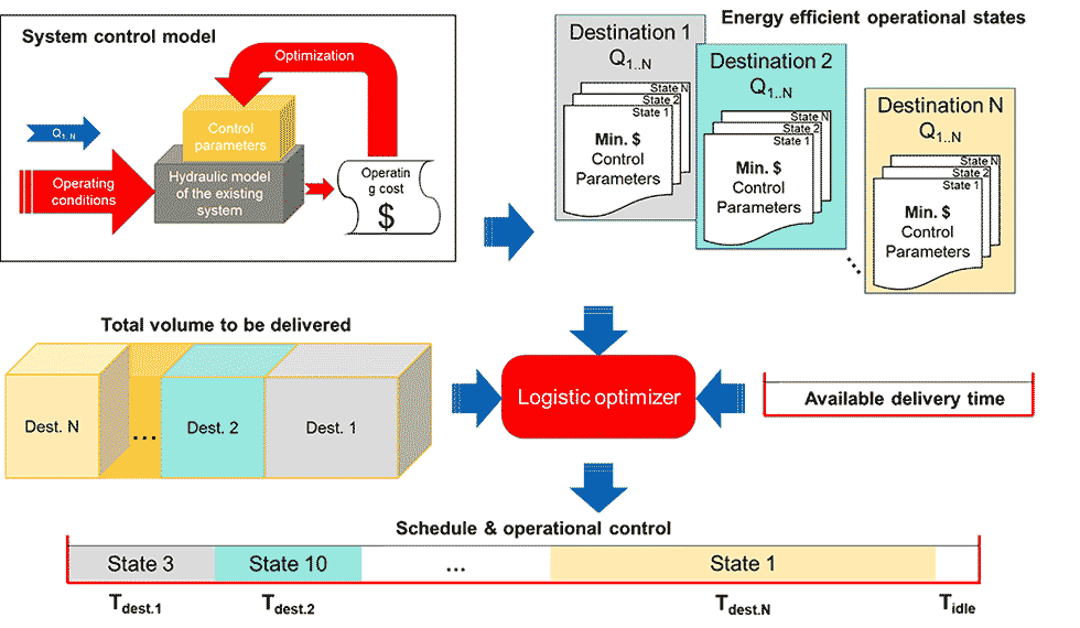
The continuous change of the DRA and energy cost however necessitates the revision of possibility of cost reduction by DRA dosing. The operator must decide on the pump combination to be used, and if applicable, the pump speeds and DRA dose for a given pumping direction. Using hydraulic optimization software, the optimal control state for any given target flow can be determined for a given destination, resulting in an operating cost-flow (opex-q) diagram.
Based on the opex-q diagrams of all destinations (Image 2), it is possible to select the combination of transport modes with the lowest overall cost in the given time frame. The energy efficiency of pumped systems can be improved mainly with improving pumps to better fit the system and adopting more efficient control methods, which requires systemwide process modeling and optimization. In the case of complex hydraulic systems, even the identification of the most favorable control parameters requires a system model-based optimization procedure.
When determining the optimal design parameters, several operating conditions with different durabilities must be considered, in which it is necessary for each to determine the optimal control parameters. The average operating cost characterizing the system can be defined as the weighted average operating cost of the possible operating conditions. In the case of energy retrofits, in addition to the operating cost, the investment cost of the conversion and the remaining lifetime of the system must be considered, based on which the optimal solution can be selected by minimizing the lifecycle cost or payback time.
References
Anderson, H.H., 1980, “Prediction of Head, Quantity and Efficiency in Pumps-The Area Ratio Principle,” Performance Prediction of Centrifugal Pumps and Compressors, ASME 22nd Annual Fluids Engineering Conference, March 9-13, New Orleans, LA, USA
The Hydraulic Institute, 2018, “Pump System Optimization: a Guide for improved energy efficiency, reliability, and profitability, second edition”
“Expert Systems for Diagnosis and Performance of Centrifugal Pumps,” Finnish Technical Research Center report, 1996.
“U.S. Industrial Motor Systems Opportunities Market Assessment,” U.S. Department of Energy, Oak Ridge National Laboratory, Xenergy, Inc., December, 2002.
Epp, R.; Fowler, A.G. Efficient code for steady-state flows in networks. J. Hydraul. Div. Am. Soc. Civ. Eng. 1970, 96, 43–56.
“Particle Swarm Optimization for Single Objective Continuous Space Problems: A Review,” Mohammad Reza Bonyadi, Zbigniew Michalewicz, Evolutionary Computation (2017) 25 (1): 1–54.
Ridao, M. A. (2004, October). “Optimal use of DRA in oil pipelines.” In 2004 IEEE International Conference on Systems, Man and Cybernetics (IEEE Cat. No. 04CH37583) (Vol. 7, pp. 6256-6261). IEEE.