Part 1 of this series (Pumps & Systems, September 2015, online here) discussed the engineering principles that dictate the operation of various elements of a piping system. Using those principles, we built a mathematical model of the example piping system based on information supplied by the equipment manufacturers and design data about the tanks and pipelines. This model can be used to simulate the operation of the physical piping system under any expected operating condition. Once the model is available, the next step is to gather the plant's operating data, which is broken down into system boundary parameters and operating results, to compare it with results of the system model. Figure 1 depicts the model piping system with plant operating data listed next to the installed instrumentation. The installed instrumentation consists of the supply tank level, the destination tank level and pressure, the pump suction PI-100 and discharge PI-101 pressures, the position of the control valve, and the flow meter FT-101, which is part of the flow control loop.
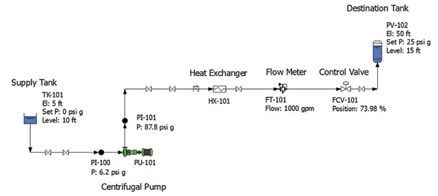 Figure 1. Piping system with plant operating data (Courtesy of the author)
Starting Energy
The starting energy of the system can be calculated by converting the tank level to feet of fluid using the Bernoulli equation. In this system, the datum elevation is set a 0 feet. Equation 1 can be used to determine the energy at the liquid level in the supply tank.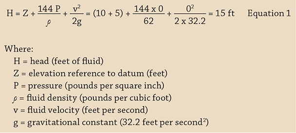
Pressure at PI-100
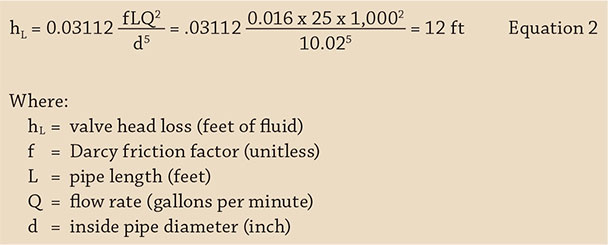
With a starting total energy of 15 feet in the supply tank and a head loss of 0.35 feet of fluid in the pipeline, the total energy at the PI-100 is 14.65 feet of fluid. Using the Bernoulli equation, we will calculate the static pressure (the pressure displayed on pressure gauges) at location PI-100. The elevation of PI-100 is 0 feet above the datum. The velocity of the fluid in a 10-inch schedule 40 steel pipe with a flow rate of 1,000 gallons per minute (gpm) is 4 feet per second. Substituting the values into the Bernoulli equation and solving for P results in a static pressure of 6.2 psig (see Equation 4) .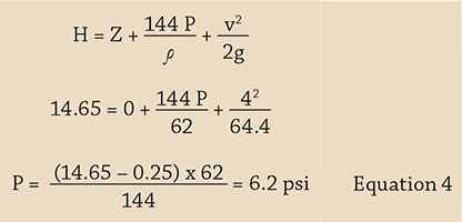
Looking at Pump PU-101
Next we will look at the operation of the centrifugal pump PU-101. Figure 2 displays a copy of the manufacturer's pump curve.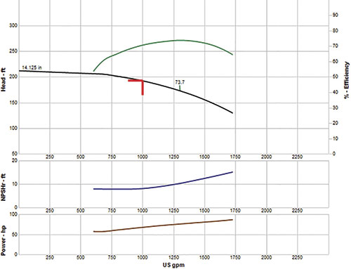 Figure 2. Manufacturer's pump curve for the centrifugal pump
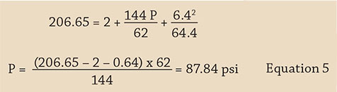
Calculating the Control Valve Inlet Energy
Next, we will calculate the total energy at the inlet of the heat exchanger. The pipeline from PI-101 to the inlet of HX-101 is 250 feet of - inch schedule 40 pipe, with two gate valves, one swing check valve with an angle seat and four long radius elbows. Using the Darcy equations as outline previously, the head loss in the pipeline is 5.46 feet of fluid. Subtracting the head loss from the total energy at PI-101 results in 201.19 feet of total energy at the inlet of HX-101 (206.65 – 5.46). Because the model does not have a pressure gauge at the inlet of HX-101, we will not be able to validate the calculated results. Next, we will determine the head loss across the heat exchanger HX-101. The heat exchanger manufacturer provided a graph that shows the head loss across the heat exchanger as a function of the flow rate (Figure 3).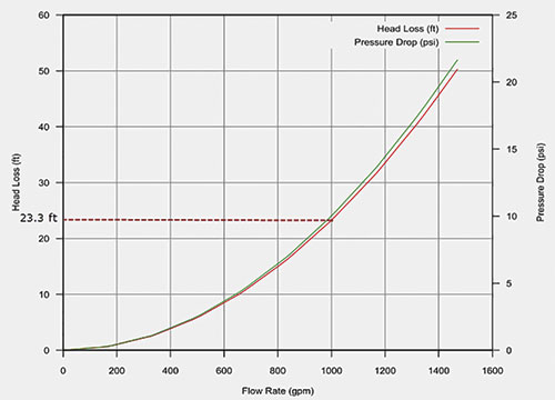 Figure 3. The manufacturer supplied head loss as a function of flow rate through heat exchanger HX-101.
Determining the Control Valve Outlet Energy
The control valves outlet energy can be determined in two ways. One method is to calculate the head loss across the control valve using the flow rate and Cv value (based on the valve manufacturer's operating data). Then, continue down the pipeline connecting the outlet of the control valve to the destination tank. The resulting energy of the fluid going into the destination tank PV-102 can be validated based on the static head (level and pressure) in the destination tank. The second way to find the head loss across the control valve is to determine the total energy at the destination tank and work upstream until reaching the outlet of the control valve. The difference in the total energy between the control valve inlet and outlet is the head loss across the control valve. We can then convert the head loss across the control valve to a differential pressure. With the control valve differential pressure and the flow rate through the valve, we can determine the Cv required. We can then compare the valve position calculated using the sizing equation and manufacturer's data to the actual valve position. If they match, then the control valve can be validated. For the purposes of this article, we will use the second method: determining the total energy at the destination tank and working upstream.Calculating the Total Energy at the Control Valve Outlet
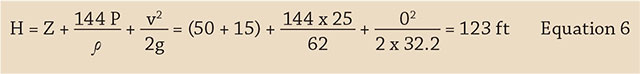
The base of PV-102 is 50 feet above the datum, with a tank level of 15 feet above the tank bottom, and the pressure above the liquid level is 25 psi. Using the Bernoulli equation, we can determine the total energy at the destination tank (see Equation 6). The head loss for 1,000 gpm in the pipeline connecting the outlet of the control valve to the inlet of the destination tank is 5.47 feet. The pipeline length is 280 feet of 8-inch schedule 40 steel pipe with a gate valve, three long radius 90-degree elbows and pipe exit into a tank.