Last month, we covered the first two parts of calculating the system resistance curve, which are total static head and pressure head. These two parts of the total equation are both flow independent. This month, we will address the third and more difficult component, the friction head curve, which is flow dependent. Do not confuse the terms dependent and independent with variable and constant.
For our calculations, we will assume the liquid properties are Newtonion, meaning the viscosity will not change with the flow rate and we are only considering circular pipe.
Plan B
Before we start, I am compelled to share that there are several online calculators and apps available to assist you with the calculation of the system resistance curve. There are also premium programs (commercial software) available at cost. The commercial software is especially helpful when you encounter sophisticated systems with branch circuits, circuits of various pipe sizes, parallel pumps, nozzles and numerous components, such as heat exchangers, that require variable thermal balancing. The apps and calculators are normally free but have limits and are restricted to simple systems. To the uninitiated, the cost for the commercial program may seem expensive, but, in my experience, they are worth every penny. When you consider the price for the premium program, you must also weigh the risk and the existential cost of not doing it correctly. Regardless of price, if you are going to use any of the apps or programs, it is still important to understand the concepts behind the basic processes, and this column can help you whether the process is manual or computerized.
Entropic Toll Road
When you force a liquid at a specified flow rate through some length of pipe, there is always resultant friction (measured in feet of liquid) that must be overcome to accomplish the process. The friction is due to the viscous shear stresses in the liquid and the interior surface roughness of the pipe. Think of the flow process like a toll road in that, for a given pipe diameter and length, there is an associated cost to pump a specified volume of liquid per unit of time. The system’s toll, like any tax, must be paid to the laws of science and nature, and there is no way to circumvent the charge. However, there are clever methods to mitigate the toll such as choosing the proper pipe diameter and materials of construction. Another way to reduce the toll is to design the system for geometric simplicity. Straight runs of unencumbered pipe are as close to an express lane as you can get on this toll road. All components in the piping system will also require an even higher toll than the piping. Elbows, valves, tees, strainers, heat exchangers, reducers, nozzles and even changes in pipe size will all require their dues. Mitigating friction tolls simply requires a minimization of total fittings and/or choices for more efficient components. An example of this could be long radius elbows versus short radius. There are also efficient component and piping geometry choices like wyes in lieu of tees and full ported valves where possible/practical.
Methods, There Are Three
There are three common methods to calculate the friction curve for your system:
K factor (resistance coefficients) normally stated as K.
Cv (flow coefficient)
Equivalent Length Method (L/D). Units are feet and the symbol = Le
We will focus on the equivalent length method in this column. It is the simplest approach and will yield reliable results if performed correctly. Caution: The equivalent length method can sometimes result in a system curve that appears more restrictive on paper than it actually is, especially if the liquid velocities fall into the lower laminar regions. Consequently, this method may yield a pump choice that is bigger than necessary. If you understand the risk, you can mitigate the issue.
The K factor approach will yield incremental accuracy over the equivalent length method, but the calculations are more tedious. The K factor approach will be the more accurate of the two approaches; the degree of accuracy depends on the system design and the corresponding range of liquid velocities.
We will not discuss the Cv method in any detail except to state that it is useful for determining pressure drops across components such as strainers, nozzles and orifices. I briefly explained flow coefficients in my January 2019 column, and you can find more information in the references at the end of this column.
This column is a 101-level discussion, so we will not delve too deep or at all into Moody diagrams, Euler, Colebrook, Navier-Stokes, Reynolds Numbers, Darcy-Weisbach or Hazen-Williams formulas. You should be aware of these principles and formulas at the 101 level. Later, as you move to the higher levels of calculating system friction, a full understanding will become mandatory to master these processes.
Additionally, please understand the viscosity of the liquid, the age of the pipe and the cleanliness/roughness of the interior pipe surface (think corrosion, dirt, fouling and marine growth) are all factors that will affect the friction factor.
Friction Loss Formula
Formula 1
Friction Head= hf=f L/D V2/2g
In the friction formula above, hf represents the friction head.
f = friction factor is a dimensionless number (Moody or Colebrook friction factor)
L = length of the pipe in units of feet.
D= diameter of the pipe. Note the units are feet not inches.
V = the average velocity of the liquid in feet per second
g = is the gravitational constant = 32.17405 feet per second squared.
Pointing out the obvious in the friction factor equation, you can see that the length of pipe imposes a direct relationship to the friction head. The longer the pipe, the more the friction factor will increase. The pipe diameter has an inverse relationship, meaning the smaller the pipe diameter, the more friction will increase. The velocity of the liquid is a square function, so you can surmise that the friction increases exponentially with flow rate, and the friction curve will be quasi parabolically shaped (technically half of a parabolic). The one factor in this equation you will have difficulty with is determining the value of f, the friction factor.
For a new system, in theory, you could determine the entire friction curve mathematically by use of the friction formula referred to as Darcy-Weisbach (a.k.a. Fanning formula). If the exact value of the f factor in the formula was known, then it would be an easy and accurate calculation. The issue is that the accuracy of the f factor value is difficult to determine because liquid viscosities, velocities and internal pipe surfaces (roughness factor ϵ) are not constant factors. Note that the Darcy-Weisbach formula is used for new pipe, and the Williams and Hazen tables are based on 10-year or older pipe.
Reynolds Number
The Reynolds number (Re) is a ratio of the liquid’s inertial forces to the viscous forces. Note that Re can also apply to gases. Because it is a ratio, it is dimensionless, and there are no units. Calculation of the Reynolds number helps to predict fluid flow patterns that tell you if the flow will be laminar, transitional or turbulent. Being able to predict where the transition from laminar to turbulent flow occurs can make a big difference in accuracy when calculating the friction head for a system.
Formula 2
Friction factor for laminar flow: f=64/Re=64/2,000=0.032
Simplification example: the friction factor can be simplified to 64 divided by the Reynolds number (denoted as Re in the formula). For typical laminar flow, the Reynolds value is 2,000. The result of 0.032 is about mid-range, and if you are stumped or guessing, it is a good choice until better information is found.
Moody Chart/Diagram
If you know the liquid velocity, pipe size and internal surface roughness, then you can estimate whether the flow is laminar or turbulent. The Moody Chart illustrates the relationship between the friction factor, the Reynolds number and the roughness of the internal pipe surface. The Moody Chart is convenient for friction calculations and to predict pressure drop or flow rate in a pipe, but it requires moderate training.
Velocity & Friction
You can calculate the liquid velocity in the pipe from a formula. Alternatively, the easy way for most applications is to simply look it up in an online reference chart/table under a search for “pipe friction tables” or use my preferred sources, which are the Cameron Hydraulic Data Book (CHDB) and Crane’s Technical Publication 410 (TP410)(Flow of Fluids Through Valves, Fittings and Pipe.)
Equivalent Length (Le)
Once you have the range of flowrates and all the pipe and component information (material, length and diameter), you have the foundation for calculating the friction head. Additionally, all the components
and valves can also be assigned an equivalent length.
Don’t be intimidated by all the formulas and calculations. Rather than go through the aforementioned equations and calculations, you can use the published information charts from these references to simplify creating the friction curve. You can achieve a fair amount of accuracy using this technique if the pipe is sized correctly, and you can use the liquid velocity as a guide to make that decision. As a general rule of thumb, if the velocity exceeds 20 feet per second, the accuracy will diminish, and you should use another method or a friction calculator program.
From the friction tables, you can garner the head loss per 100 feet of pipe if you know the flow rate, pipe material and size. Head losses are normally expressed as X amount of loss in linear feet per 100 feet of pipe.
Example: From a friction chart, we see that 400 gallons per minute of water moving through a new 4-inch schedule 40 steel pipe would create a head loss of 8.51 feet per 100 feet of pipe. Using that information, in an example with 500 feet of pipe the friction loss due to the piping would be 8.51 x 500/100=42.55 feet.
Realize that any components such as valves, tees and wyes have to be calculated separately for friction loss and then added, which is the next step.
Pipe system components, such as valves and fittings, have K and Cv numbers, but they also have equivalent length values (units of linear feet) that you can look up in tables/charts in the references. Let’s assume that all the fittings are 4 inches for our example. For a given type and size of component, there is a head loss stated in equivalent length of straight pipe and units of feet. For example, a 4-inch gate valve that is fully open has a typical loss of the equivalent of 2.6 linear feet of 4-inch pipe. You can continue and look up all the other 4-inch components in the system and record their equivalent lengths. Subsequently, add the equivalent lengths for all of the components to get the total. Now, with that total number for the components, you can add that value to the total piping length, previously stated as 500 feet.
What we don’t know at this point is the actual range of flow rates, but what we do know is that mathematically it takes a minimum of three points to determine a curve. I like to have more than three points, and 4 or five will suffice for the example where we already know that the shape of the curve will be approximately parabolic. The first flowrate, and hence the first curve point, will be at dead head, so it is zero flow corresponding to no friction loss. The second point should be around 30% of the expected flow, the third point at 70% and the 4th point at 110%.
Example
For our simple system example of 500 feet of 4-inch steel pipe, we should also assume that there are two fully open gate valves, a quantity of 4 long radius elbows and one open swing check valve. All component port diameters are a nominal 4 inches. Technically you should always use the actual internal diameter of the pipe or component. We are just solving for the friction curve at this point. We will also assume and add a static head of 50 feet and zero pressure head. The friction loss for a given system depends on the flow rate. Friction losses used are from the tables (Page 3-134 CHDB)
Pipe: Given 500 feet of 4-inch schedule 40 steel.
Gate valves (4 inches) (quantity two) at 2.6 feet each for a total 5.2 feet
Swing check valve (4 inches) (quantity one) for 33 feet.
Long radius 90-degree elbows (4 inches) (quantity 4) at 4 feet each is a total of 16 feet.
Total equivalent length in feet is: 500 + 5.2 + 33 +16 = 554.2 feet ≈ 555 feet.
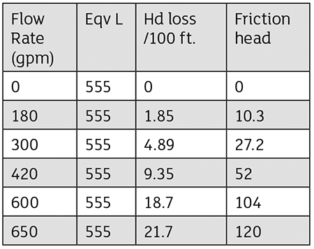
Assume expected flow rates (gallons per minute) of 0,180,300,420,600 and 650.
Enter the data in an excel worksheet or simply do the math to arrive at the friction head for each flow rate.
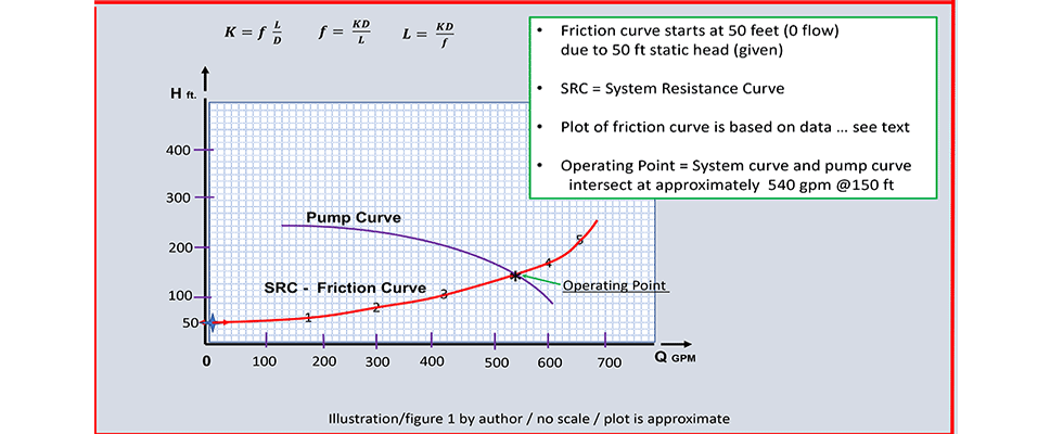
Finally, we can take these six points and plot them. Note that there is already 50 feet of static head, so the friction curve starts at 50 feet and zero flow. See Image 1.
The intent of the column is to help you figure out where your pump is operating on the system curve. When in doubt, ask for help from a knowledgeable, qualified and experienced engineer or technical person.
References
Crane Technical Publication 410; Flow of Fluids…
Cameron Hydraulic Data Book (20th edition)
The Pump Handbook (4th Edition)
Hydraulic Institute; Engineering Data Book