It is common to use graphical techniques to determine the performance of multiple centrifugal pumps operating in series or in parallel. These methods are often time-consuming and rely on the good eyesight of the person making the measurements and a steady hand while drawing the combined performance curves. Numerical techniques can be employed to determine the same overall performance of centrifugal pumps operating in series and in parallel. This article will identify the steps for using numerical techniques within an Excel spreadsheet to achieve this goal. It will provide sample calculations of those numerical techniques with detailed cell formulas so that end users can reproduce this technique in their own pump applications. For this article, it is assumed that each pump is a two-stage centrifugal pump that has different performance for the first stage compared to the second stage. These techniques can easily be extended to accommodate multistage pumps that have more than two stages.
Steps for Numerical Techniques
The individual steps are summarized below: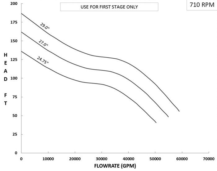 Figure 1. First stage pump performance
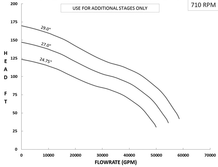 Figure 2. Second stage pump performance
- Digitize or make “rough eye” estimates to measure 10 or more (Q, H) points from shutoff to runout conditions for the first stage pump performance curve of head versus flow. Enter the array of first stage head versus flow data into spreadsheet columns.
- If necessary, use numerical methods to extend the head versus flow data beyond runout. This step is done primarily to prevent subsequent numerical methods from going off into the weeds.
- Curve fit a polynomial function to the first stage head versus flow data, which may include extrapolated data down to zero head rise.
- Duplicate steps 1, 2 and 3 with measurements of the second stage head versus flow data. Although it is not essential, it is convenient and recommended that both polynomial curve fits be of the same order.
- Determine the function of head versus flow for both stages operating together in series. This is done by adding the coefficients of the same ordered terms of the polynomial functions for each stage to establish the applicable coefficients of the polynomial function for the multistage pump.
- Determine the polynomial function for the combined performance for multiple (and identical) pumps operating in parallel. The set of coefficients for the polynomial will vary depending on the number of pumps running in parallel.
- Determine the second order polynomial function, which characterizes the resistance (head loss versus flow) of the system piping.
- Determine the polynomial function that defines overall parallel pump performance minus the system resistance function.
- Determine the derivative of the polynomial function from the previous step. The derivative function provides the slope of the head versus flow curve, which is needed in the next step.
- Use iterative numerical methods to solve for head and flow operating points of multiple parallel pumps operating within the specified system. This method uses consecutive rows of spreadsheet calculations to perform successive iterations of the Newton-Raphson method. Results of each iteration eventually converge to the solution of flow rate.
.jpg) Table 1. Head versus flow arrays for each pump stage
Table 1. Head versus flow arrays for each pump stageSample Calculations
A set of sample calculations is provided in this section to demonstrate these steps. Assume that multiple, two-stage centrifugal pumps in parallel are used. Assume that the first stage performance is shown in Figure 1, and second stage performance is shown in Figure 2. Assume that both stages of each pump are equipped with a 29-inch impeller, corresponding to the top head curve shown in Figures 1 and 2. The head curves for each stage were digitized, and the resulting arrays are provided in Table 1. This same data could have also been determined by visual inspection and likely with fewer decimal places. It should be noted that the number of decimal places shown does not imply any more or less accuracy of the calculations based on such data, because the native spreadsheet stores more decimal places than those that are shown. The head versus flow arrays (see Table 1) for each stage can be fitted with a polynomial function that has sufficient order to provide a reasonably accurate representation of the data. For demonstration purposes, assume an eighth order polynomial that has the form shown in Equation 1 that gives the head rise in feet (FT). Where:
Q = Flow rate (gallons per minute)
Coefficients a, b, c, d,e, f, g, h and j = Constants determined by Excel spreadsheet equations using INDEX() and LINEST() functions
Units for each coefficient are FT per gpm raised to the same power as the flow rate within the same term. Separate sets of coefficients applicable for each stage will be determined. Coefficient subscripts 1 and 2 will be used to distinguish between Stages 1 and 2, respectively.
Where:
Q = Flow rate (gallons per minute)
Coefficients a, b, c, d,e, f, g, h and j = Constants determined by Excel spreadsheet equations using INDEX() and LINEST() functions
Units for each coefficient are FT per gpm raised to the same power as the flow rate within the same term. Separate sets of coefficients applicable for each stage will be determined. Coefficient subscripts 1 and 2 will be used to distinguish between Stages 1 and 2, respectively.
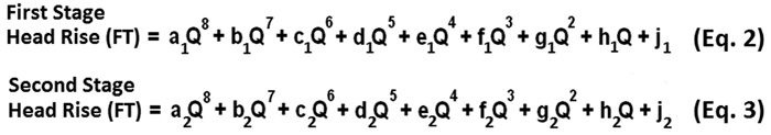
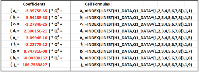 Table 2. Polynomial coefficients and associated cell formulas for first stage, Equation 2.
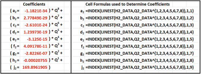 Table 3. Polynomial coefficients and associated cell formulas for second stage, Equation 3
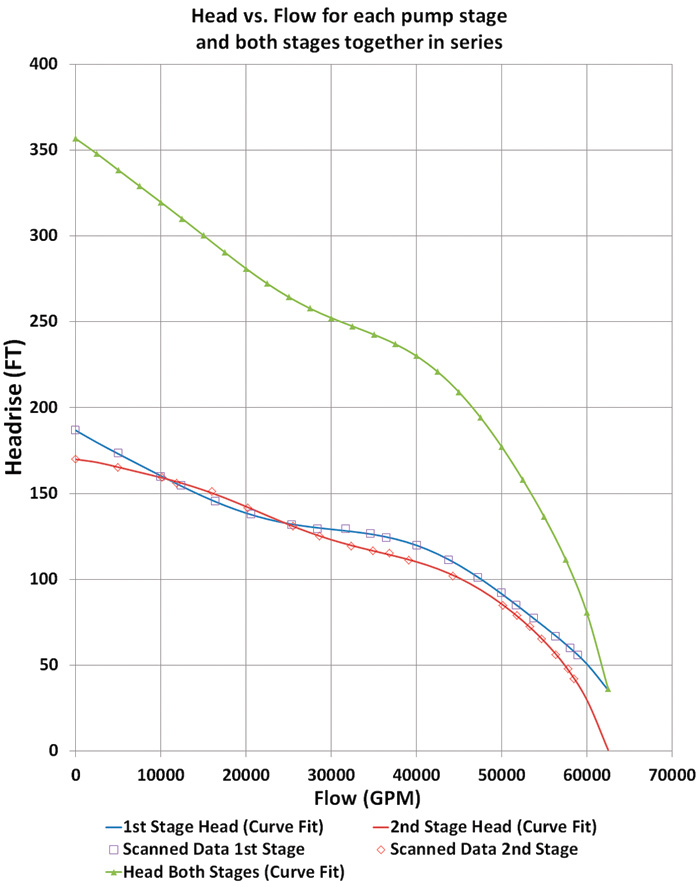 Figure 3. Plot of single pump, head versus flow
- Range name of “Q1_DATA” will be assigned to the first stage flow rate values shown in the first column of Table 1.
- Range name of “H1_DATA” will be assigned to the first stage head rise values shown in the second column in Table 1.
- Range name of “Q2_DATA” will be assigned to the second stage flow rate values shown in the third column of Table 1.
- Range name of “H2_DATA” will be assigned to the second stage head rise values shown in the fourth column of Table 1.
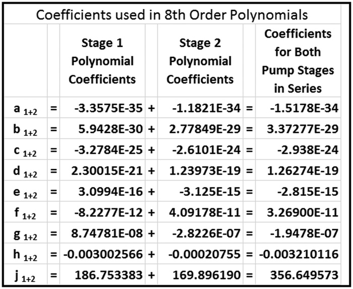 Table 4. Polynomial coefficients and associated cell formulas for Stages 1 and 2
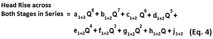 If the plotted region beyond runout for the polynomial functions of head versus flow for either stage includes a relative minimum and curve back up, then it is recommended that end users include an additional data point at the end of the head flow array to force the polynomial curve fit to be concave downward. The fabricated data point should have a head rise of zero at a flow rate slightly beyond runout. The use of a fabricated data point beyond runout does not imply any accuracy regarding the pump performance in that region. The sole purpose of this fabricated data point—if one is used—is to improve the stability of the numerical methods that are demonstrated later and that pertain to parallel pump operation within a system.
If the multistage pump happens to include more than two stages and those additional stages are identical in performance to the second stage, then the second stage polynomial coefficients can be multiplied by the integer number of stages beyond the first stage. The coefficients can then be summed with the same ordered coefficients associated with the first stage to determine the polynomial coefficients for the entire multistage pump.
If the plotted region beyond runout for the polynomial functions of head versus flow for either stage includes a relative minimum and curve back up, then it is recommended that end users include an additional data point at the end of the head flow array to force the polynomial curve fit to be concave downward. The fabricated data point should have a head rise of zero at a flow rate slightly beyond runout. The use of a fabricated data point beyond runout does not imply any accuracy regarding the pump performance in that region. The sole purpose of this fabricated data point—if one is used—is to improve the stability of the numerical methods that are demonstrated later and that pertain to parallel pump operation within a system.
If the multistage pump happens to include more than two stages and those additional stages are identical in performance to the second stage, then the second stage polynomial coefficients can be multiplied by the integer number of stages beyond the first stage. The coefficients can then be summed with the same ordered coefficients associated with the first stage to determine the polynomial coefficients for the entire multistage pump.
Multiple Pumps Operating in Parallel
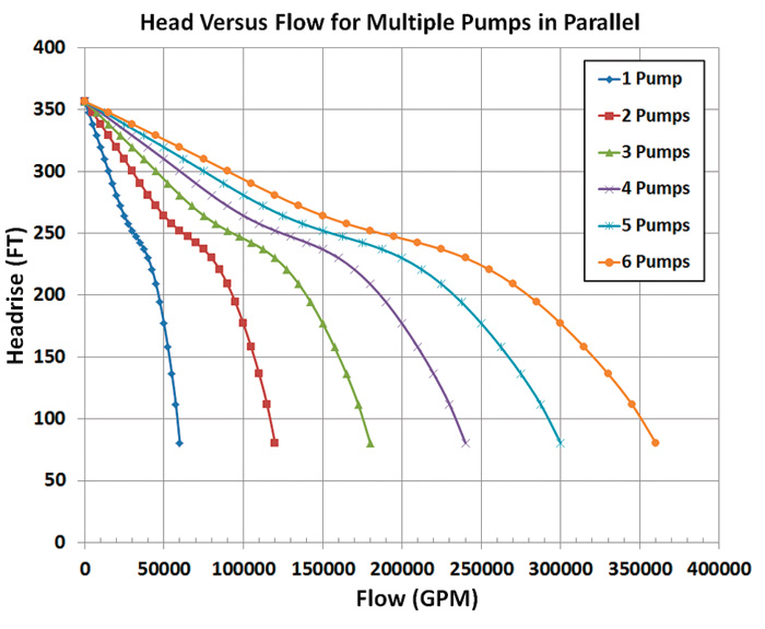 Figure 4. Plot of parallel pump performance
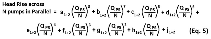 Where:
QPS = The total flow rate through the pump station
N = The number of pumps running in parallel
a, b, c, d, e, f, g, h and j = Previously determined polynomial coefficients
1+2 = Both stages of each pump
The head versus flow performance for multiple pumps in parallel based on Equation 5 can easily be calculated and plotted in a spreadsheet. Figure 4 shows the station performance based on one to six pumps running in parallel, while the performance of each pump is shown in Figure 3.
Where:
QPS = The total flow rate through the pump station
N = The number of pumps running in parallel
a, b, c, d, e, f, g, h and j = Previously determined polynomial coefficients
1+2 = Both stages of each pump
The head versus flow performance for multiple pumps in parallel based on Equation 5 can easily be calculated and plotted in a spreadsheet. Figure 4 shows the station performance based on one to six pumps running in parallel, while the performance of each pump is shown in Figure 3.
Characterizing System Resistance
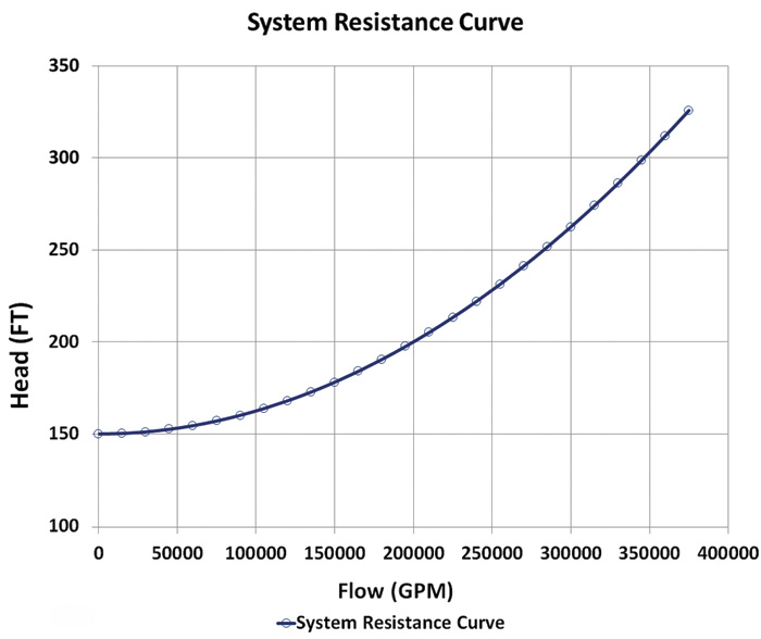 Figure 5. System resistance versus flow rate
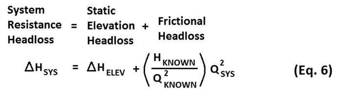 For example, assume that the downstream pipeline has a rise in elevation that must be overcome by a pump station head rise of 150 feet before the pumps will begin to flow. Also, assume that for a known flow rate of 200,000 gpm, there is a calculated or known head loss due to friction of 50 feet. Furthermore, assume that head loss due to friction is a function of the square of the flow rate, which is consistent with the Darcy-Weisbach equation. This enables end users to determine a functional relationship that defines the head loss versus flow. From the above assumptions, the functional relationship for the resistance of the example system can be defined using Equation 7.
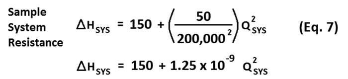 A plot of the system resistance curve based on Equation 7 is depicted in Figure 5. The shape of the curve is parabolic because head loss is proportional to the square of the flow rate.
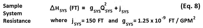
If Equation 7 is rearranged to have the same format as Equation 1, it would appear as Equation 8.
A plot of the system resistance curve based on Equation 7 is depicted in Figure 5. The shape of the curve is parabolic because head loss is proportional to the square of the flow rate.
If Equation 7 is rearranged to have the same format as Equation 1, it would appear as Equation 8.
Combining Equations
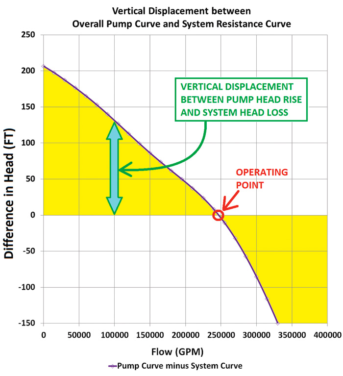
If end users plot the system resistance curve and overall pump curve on the same graph, the point at which the lines cross will designate the operating point for the pumps. For example, if six pumps run in parallel and their combined performance is shown for six-pump operation in Figure 4, then the operating point could be determined graphically (see Figure 6). If end users can develop a function of ΔHead versus flow, which quantifies the vertical displacement between the two curves as depicted by the two-headed arrow shown at a flow rate of 100,000 gpm (Figure 6), then end users can mathematically solve such a function for the point at which the two curves intersect. The applicable head difference function is obtained by subtracting the system resistance parabolic function (Equation 8) from the overall pump curve polynomial function (Equation 5). This results in Equation 9.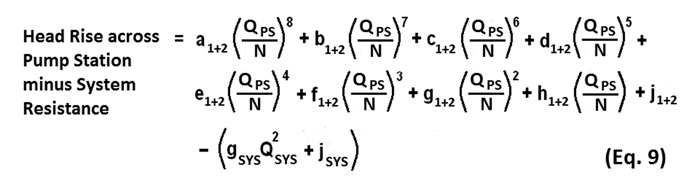 Where:
QPS = The total flow rate through the pump station
QSYS = The flow rate through the system and is equal to QPS
N = The number of pumps running in parallel
a, b, c, d, e, f, g, h and j = Previously determined polynomial coefficients
1+2 = Both stages of each pump
PS = All pumps running in parallel in the pump station
SYS = The system resistance
Where:
QPS = The total flow rate through the pump station
QSYS = The flow rate through the system and is equal to QPS
N = The number of pumps running in parallel
a, b, c, d, e, f, g, h and j = Previously determined polynomial coefficients
1+2 = Both stages of each pump
PS = All pumps running in parallel in the pump station
SYS = The system resistance
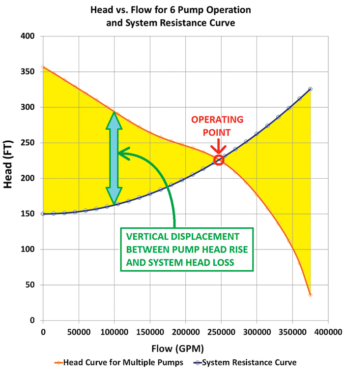 Figure 6. Overall pump curve and system curve
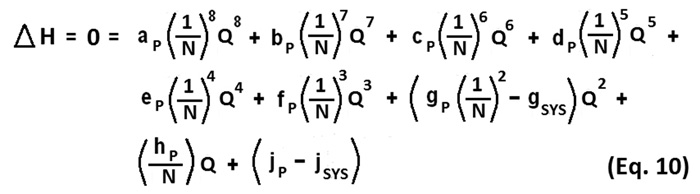
 Where:
Q = The total flow rate through both the pump station and system
N = The number of pumps running in parallel
a, b, c, d, e, f, g, h and j = Previously determined polynomial coefficients
P = Each pump within the station
SYS = The system resistance curve
Where:
Q = The total flow rate through both the pump station and system
N = The number of pumps running in parallel
a, b, c, d, e, f, g, h and j = Previously determined polynomial coefficients
P = Each pump within the station
SYS = The system resistance curve
Numerical Solution of Flow Rate
Flow rate can be determined by solving Equation 10 for a specified number of running pumps by using numerical techniques. A solution within an Excel spreadsheet is achieved by using “GOALSEEK,” in which an initial guess at flow rate is input into one cell, and another cell contains the formula shown in Equation 10. Within the “GOALSEEK” pop-up window, the user chooses to seek a value of flow rate, for which the computed head difference is zero. In rare cases, more than one mathematical solution is found. This situation may only occur if two conditions are met—the overall pump curve contains a droop such that head versus flow is not monotonically decreasing, and the system resistance curve is flat, as when comprised almost exclusively of elevation head loss with minimal friction losses. In general, it is not a good idea to design a pump station with parallel pumps that have a drooping head curve. However, if both these conditions are met and more than one solution exists, then the mathematical solution of flow rate will usually—but not always—converge on whichever value of flow is closest to the initial guess.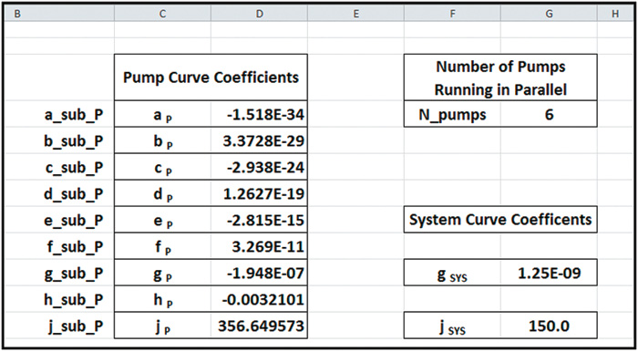
.jpg)
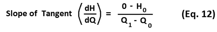
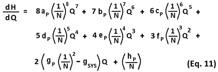 In general, the overall slope of the curve in Figure 7 should always be negative in sign throughout its range of operating flow rates. If one extrapolates the tangent line from the (Q0, H0) point on the curve to cross the x-axis, then the flow rate at which the tangent line crosses the x-axis becomes the next guess of flow rate for the next iteration. This flow rate is Q1, and the associated point on the x-axis is (Q1, 0). A tangent line segment runs between two points—Q0, H0 and Q1, 0—and the slope of that line segment is represented by the right-hand side of Equation 12. Evaluation of Equation 11 provides the value of the left-hand side of Equation 12.
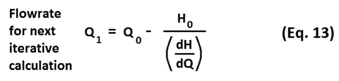
 All the terms—except Q1—in Equation 12 have known values. The terms of this equation can be rearranged to solve for Q1 as shown in Equation 13.
 Equations 9, 10, 11, 12 and 13 contain all the tools needed to construct a spreadsheet, which can calculate the flow rate through a specified system for a specified number of pumps running in parallel. Table 5 contains a summary of the input parameters, which are used within the cell formulas that are evaluated within the spreadsheet to calculate flow rate by means of the Newton-Raphson iterative method.
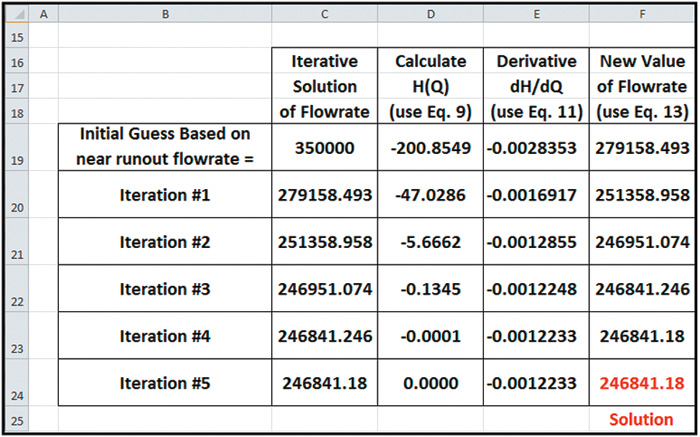
The summary of calculations shown in Table 6 demonstrates that within five iterations, the successive values of the solution flow rate had converged to within two decimal places. The display of this many decimal places is done solely for the purpose of demonstrating convergence of the solution and does not imply unjustified accuracy of the solution. The use of polynomial curve fits is an approximation.
It should also be noted that the number of iterations needed for convergence may vary depending on the closeness of the initial guess to the final solution. The number of iterations can also vary depending on the number of decimal places being considered for the testing convergence.
The cell formulas entered into columns D, E and F in Table 6 are based on Equations 9, 11 and 13, respectively. The actual cell formula syntax that can be used in an Excel spreadsheet is summarized in Table 7. Although the initial development of a spreadsheet of this nature can be cumbersome, once it is developed it can provide a useful tool for future pump performance calculations.
Equations 9, 10, 11, 12 and 13 contain all the tools needed to construct a spreadsheet, which can calculate the flow rate through a specified system for a specified number of pumps running in parallel. Table 5 contains a summary of the input parameters, which are used within the cell formulas that are evaluated within the spreadsheet to calculate flow rate by means of the Newton-Raphson iterative method.
The summary of calculations shown in Table 6 demonstrates that within five iterations, the successive values of the solution flow rate had converged to within two decimal places. The display of this many decimal places is done solely for the purpose of demonstrating convergence of the solution and does not imply unjustified accuracy of the solution. The use of polynomial curve fits is an approximation.
It should also be noted that the number of iterations needed for convergence may vary depending on the closeness of the initial guess to the final solution. The number of iterations can also vary depending on the number of decimal places being considered for the testing convergence.
The cell formulas entered into columns D, E and F in Table 6 are based on Equations 9, 11 and 13, respectively. The actual cell formula syntax that can be used in an Excel spreadsheet is summarized in Table 7. Although the initial development of a spreadsheet of this nature can be cumbersome, once it is developed it can provide a useful tool for future pump performance calculations.