08/05/2015
This series discusses the control elements of a piping system, which improve the quality of the product. Part 1 (Pumps & Systems, July 2015) covered passive controls, such as overflow and bypass controls, on/off controls, and manual controls.
Active Control Operation
Active controls maintain a set value of a process variable under changing system operating conditions. They are often referred to as a control loop (see Figure 3). The level in the destination tank is measured by the level transmitter that sends the measured value (MV) to the level controller. The desired tank level set point (SP) is entered into the controller. The controller compares the MV to the SP, and a controller output (CO) is sent to the final control element—a control valve in this case. The flow rate into the tank (Qin) is adjusted to maintain the desired tank level.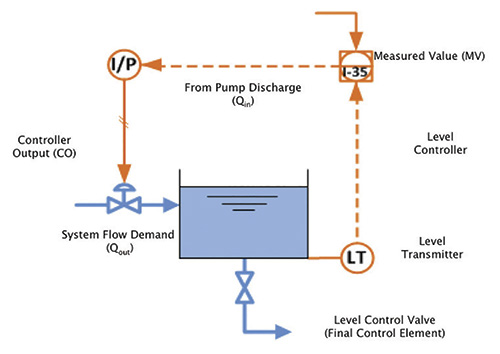 Figure 3. An example of an active control loop maintaining tank level by adjusting the flow rate into the tank (Graphics courtesy of the author)
- pump flow rate, caused by changes in the static head
- pump flow rate, caused by mechanical wear
- the flow rate out of the tank caused by a change in the system flow demand
- the tank level set point caused by the operator
Level Control with a Control Valve
The pump curve in Figure 2, Part 1 of this series (Pumps & Systems, July 2015) shows that the pump produces 125 feet of head at 400 gallons per minute (gpm). The sum of the static and dynamic head for 400 gpm through the system is 76 feet. At 400 gpm, the pump produces 125 feet of head, but the system only needs 76 feet of head. As a result, the control valve must absorb 49 feet of head to limit the flow rate to the set value. The advantage of level control with a control valve is the ability to minimize process variability by maintaining a more consistent tank level. The disadvantage is the added cost of the control loop, the need to tune and maintain the control loop, and the added head loss across the control valve necessary to maintain control. The annual operating cost of a control valve appears in Table 3.Table 3. The annual operating costs for using a control valve to control the flow. This is the same operating cost calculation for the manual control.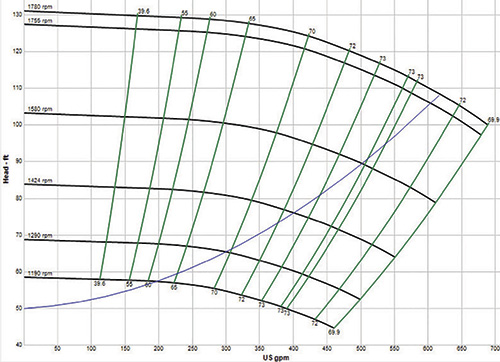 Figure 4. A pump system curve showing the pump operating at various speeds. The pump operating at 1,424 rpm provides 76 feet of head, equal to the process requirements at 400 gpm.