Introductory pump sizing courses provide foundational knowledge and familiarization with terms but do not provide the full picture. A design point, though critical in selecting a pump, is only one piece of the puzzle. To fully understand the relationship between flow and pressure in a system and how a pump interacts with that system, additional information is needed. The system head curve gives the full picture that a single design point fails to and provides additional information to select the best equipment for each application.
For the purpose of this article, the system in system head curve is defined as the pipe, number and type of valves, static head, and any other aspects of the design that may affect the pressure on the pump. The system head curve is a graphical representation of how the pressure changes as flow changes through the system. In a sense, the system head curve is the performance curve of the piping network. Pump sizing software calculates the system head curve based on user inputs, though it can be calculated in workbook applications like Excel or estimated by calculating the total dynamic head (TDH) at various flow rates and drawing a line of best fit through them. In the wastewater industry, system head curves are most commonly calculated using the Hazen-Williams equation; however, other methods and equations do exist.
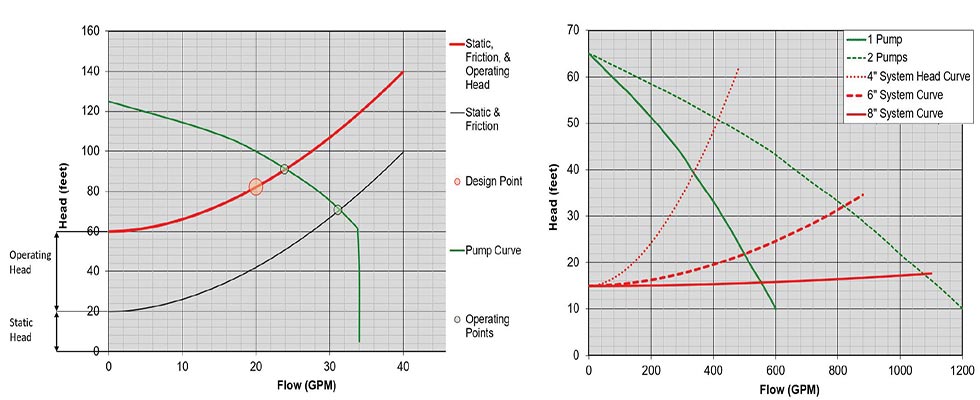
System head curves are unique to each application, but understanding how they are created can give some quick information. Generally, they are in the shape of a half-parabola. The magnitude of the exponential curve is related to the friction loss. The more friction loss a system has, such as in undersized pipes, the steeper the system head curve is. The less friction loss a system has, such as in oversized pipes, the flatter the system head curve is. The Y-intercept of the curve is the static head because at a flow of zero gallons per minute (gpm) there is no friction loss, only static head. If there is an additional operating head requirement, such as tying into a force main, the additional operating head can be modeled by shifting the Y-intercept up (static plus operating head). See Image 1 for an example of the various components of a system head curve.
There are multiple benefits and information that can be provided by the system head curve that cannot be addressed in a single article. This article will address some of the benefits the system head curve can provide such as determining operating points, analyzing simultaneous operation, piping design, variable frequency drives (VFDs), varying design conditions and comparison of conservative and expected performance.
Determining Operating Points
A pump will only operate along its performance curve. However, many times the design point used to select a pump is not on the pump’s performance curve. The question may be asked, “what flow will the pump produce?” The system head curve provides the answer. The intersection of the system head curve and the pump’s performance curve is the operating point. The operating point defines the system head and flow rate, the flow and pressure the pump will produce in that system. In Image 1, the design point is 20 gpm at 82 feet TDH. Without the system curve, it could be determined that the pump in the graph would be acceptable, but the flow produced by the pump would not be known. However, the system curve indicates the operating point of 24 gpm at 91 feet TDH. The operating point is another valuable piece of information that should be used in place of the design flow in other aspects of system design such as control set points (off, lead, lag and more), cycle times, basin sizing, etc. The operating point will also define the estimated efficiency point.
Simultaneous Operation
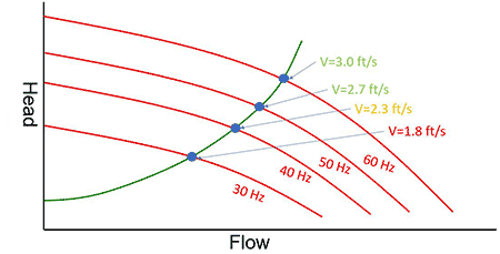
It is commonly mistaken that two pumps operating in parallel will double the flow of what a single pump can produce by itself. This would only be true if both pumps had independent and identical piping networks between the pump and outfall. However, it is common in multipump lift stations to have a single, common header and discharge for all pumps. To fully understand and compare the performance of a single pump and multiple pumps operating simultaneously, the system head curve must be used. Image 2 shows the performance curve of a single pump, a composite curve of two pumps operating simultaneously and three system curves at various diameters. Image 2 demonstrates the system head curve and allows users to better understand how a single pump compares to multiple pumps operating simultaneously. Additionally, Image 2 demonstrates the ways manipulating the piping network can affect operating points and allows the designer to dial in a more favorable operating point.
Variable Frequency Drives
VFDs are great in the proper applications. VFDs can reduce energy consumption, reduce the number of starts, quickly adapt to varying incoming flow rates, reduce wear and tear with soft starts—the list goes on. So, why not use them on all pumps? The first reason is cost and the second is application-based. The system head curve will help with the latter. Image 3 is a representation of a pump’s performance at varied frequencies. The system head curve and operating points look ideal at first (however, in sewage applications the velocity must be greater than or equal to 2 feet per second [ft/s]). The operating point when running the pump at 30 hertz (Hz) will drop the velocity below that minimum. This does not mean a VFD is not viable in sewage applications, but the minimum frequency should be set so that the pump can exceed the minimum scouring velocity. Additionally, VFDs can be less viable in systems where the static head is greater than 50% of the TDH or on systems with flat system head curves.
Applications With Varying Design Points
System head curves are also great for evaluating applications with varying design points. Some examples of applications with varying design points are pipe systems that partially, or entirely, drain between pump cycles (high points, pumping downhill, etc.), deep basins with varying water levels and static head, pressure sewer (peak flow versus nonpeak flow), and other specialty applications. In the event an application has varying design points, it is best to select a pump that can safely and adequately operate at each design point. The system head curve provides the clarity needed. For example, Image 1 has two system head curves, one that models the static and friction loss from the pump to a force main (lateral losses only) and another that models the static, friction and operating head of the force main (lateral losses plus force main pressure). In the event there is no pressure on the force main, which is possible in off-peak times, the pump will operate at the higher flow, lower head operating point. In the event the pressure in the force main is at its peak, the pump will operate at the lower flow, higher head operating point. The two separate system head curves and pump curve establish the extreme operating points. Since the extreme operating points and the entire pump curve in-between is at a safe operating point on the pump curve, this pump is a viable option. If either of the system curves does not intersect the pump’s performance curve at a desirable flow or operating point, a different pump should be analyzed.
Conservative vs. Expected Performance
It can be helpful to evaluate a design condition versus the expected condition. Many regulating authorities require the use of conservative values, such as a C-value of 120 for friction loss calculations, which can have a significant impact on designs with extended runs of pipe or high friction loss. It is generally best practice to buffer a design with conservancy and factors of safety, and it is not the author’s recommendation to abandon this practice. It is recommended for those designing pumping stations to reach out to their local regulating authority to ensure their design complies. However, it is beneficial to look at the expected, nonconservative case as well. If only the conservative case is analyzed, once installed, the pump may run further out on its curve than anticipated due to lower pressures. The actual operating point could be less efficient and increase amp draw. It may be beneficial to evaluate the pump selection with two system head curves, one with conservative values and one with expected values, and select a pump that can operate adequately at both operating points.
In conclusion, the system head curve can provide many insights into proper pump selection. System head curves provide a deeper understanding of how the piping network influences the performance of the pump and the system. When sizing a pump, be sure to check the system head curve to fully understand how the system will operate and what can be adjusted to provide the best solution.