Drives with active energy control can save energy and extend motor life for pumping and HVAC loads.

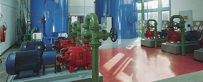
NASA Tech Briefs describes proportional integral derivative (PID) controllers as "the modern industrial workhorse" because of their distinct role in automating the regulation tasks of today's advanced process control systems. PID controllers are well-suited for many speed, temperature, flow and pressure processes. In industrial and commercial settings where these elements are sometimes matched with processes that are nonlinear, that exhibit high inertia or that require multiple complex calculations, PID control can add significant value, automating many operations that would otherwise need to be performed manually.

Yet, for many hydronics and heating, ventilating and air-conditioning (HVAC) applications that use induction motors to power pumps and fans, the torque needed to drive the motor loads varies based on the shaft speed of the motor, which can be controlled by a variable frequency drive (VFD).

Leveraging advanced VFD algorithms for PID-controlled applications in industrial and commercial building settings is a unique approach that can improve the longevity of electric motors and reduce energy consumption for systems.

Tuning into Control Modes

PID controllers regulate output through the sum of their proportional, integral and derivative actions. Most control loops require proportional and integral methods, while motion control responds best to derivative methods. Temperature regulation often requires a mix of all three. The following descriptions highlight the differences between each type of control.

Proportional control simply matches output action to error proportionally.

In integral control, the controller reduces errors through incremental or decremental outputs that gradually improve or refine the overall process. The speed with which this occurs can be fast or slow depending on whether the error is large or small, respectively. But the integral timing must be precise to avoid problems in the loop, such as sluggishness or instability.

BRIEF DESCRIPTION OF IMAGE

Derivative control provides faster, more responsive output action, but it is also highly sensitive to measurement noise. For this reason, it is used more selectively. Derivative controllers measure an adjustable time setting in minutes and seconds and derive the amount of output action to be produced based on that measurement. In other words, the controller reduces errors by calculating outputs against an observed rate of change. As the rate of change increases, more or less control is exerted. Instability can result if the derivative time is set too long.

Timing and tuning are paramount to achieving both optimal efficiency and high performance with PID controllers. This is why VFDs can often provide important support for process controls.

In the example of pumping and HVAC applications, the relationship between the shaft speed and the other key parameters for a pump or fan is expressed in the affinity laws: Flow is proportional to shaft speed, head/pressure is proportional to the square of the shaft speed, and power is proportional to the cube of the shaft speed. Based on these affinity laws, the torque needed to power a fan or pump at a lower reference frequency is lower than that required for a higher reference frequency.

The main benefit of reducing the input voltage to an induction motor is the consequent reduction in motor core losses, which are typically proportional to the square of the input voltage. Applying unnecessarily high voltage to the motor generates excessive motor core losses in the form of heat and noise.

In fact, noise and variability are the primary challenges for PID controllers. If the controller creates volatility in the process, efficiency will suffer and unnecessary wear and tear is likely to occur.

Most PID controllers require tuning to time the speed of the output action properly. Some tuning rules, such as Cohen-Coon, work well on almost all control loops that require a rapid response. But even with this approach, additional methods are still needed to address concurrent impacts on oscillation. In addition, tuning rules do not always work well with self-regulating processes that stabilize at a point of equilibrium.

To meet the specific objectives for each aspect of PID control, hundreds of controller-tuning methods have evolved. Two examples of PID-control designs include noninteractive and parallel algorithms.

Active Energy Control

One specialized energy control algorithm optimizes energy usage to produce 2 to 10 percent energy savings over standard drives.

A standard drive controls a motor based on a linear volts-per-hertz (V/Hz) relationship. The output voltage waveform of a standard VFD is typically based on pulse-width modulation (PWM). The amplitude, duty cycle and periodicity of the PWM waveform decide the effective voltage and frequency of the VFD output.

In contrast, a VFD using the active energy control algorithm dynamically adjusts the voltage down at a given reference frequency, successfully automating reduced voltage while maintaining the optimal torque and speed performance of the motor. No manual tuning is required. Instead, the algorithm dynamically adjusts the motor's operating point based on its load conditions, providing power savings and improving energy efficiency.

Both linear and square/quadratic V/Hz curves are static V/Hz control methods, which means that the voltage output depends only on the reference frequency without any considerations based on the actual motor load. If the motor load is low, the static voltage generated by either curve may be more than adequate to power the load, generating unnecessary core losses. However, if the motor load is higher than what the static voltage can handle, the squared V/Hz control method may endanger the motor's stability and cause it to overheat or stall.

These concerns are the major motivation for the design of dynamic V/Hz control methods. The active energy control method takes into account the motor's real-time operating parameters when determining the output voltage of the VFD. The control algorithm monitors the motor load and motor current, as well as other parameters, to find an operating point that both optimizes energy usage and ensures motor stability.

This algorithm is built into the logic of the drive. Upon drive startup, the algorithm begins to analyze the demand using the factory default setting for V/Hz mode.

Once the drive is given a run command, it outputs a given reference frequency and voltage level, which is determined based on the initialized V/Hz relationship. If that reference frequency is steady, the drive will start to back down the output voltage in 5 volts alternating-current (VAC) increments to determine if the motor can still provide the same torque output required at a lower voltage.

To ensure the stability of the motor, the algorithm initially sets the drive output voltage at the same level as the voltage based on the linear V/Hz method for the same reference frequency. It then begins to reduce the voltage incrementally to optimize energy usage. Meanwhile, the algorithm monitors several real-time parameters to prevent the motor from conditions that may lead to instability. When the motor enters the optimal zone of operation, the drive output voltage stays the same until commands to the drive trigger a change. After the output voltage stabilizes, the drive continues to monitor the real-time parameters of the motor to prevent instability.

If the motor output frequency remains constant, the drive will continue to reduce the motor voltage until the output frequency becomes unstable. Once the drive hits the unstable region, it will bump the voltage up 10 VAC to let the torque stabilize and maintain that level.

If the reference frequency or the stability of the load changes, the voltage will dynamically adjust back to following the linear V/Hz scale. The process repeats itself automatically each time the frequency is changed. With the load held at a constant speed, the voltage reduced and the current increased during this process, the system can capture significant power savings because of the reduction in motor core losses.

Efficiency & Cost Savings

In a comparison of this active energy control algorithm over linear V/Hz control, an unloaded, low-horsepower rated motor with an output frequency of 30.00 Hz, 885 revolutions per minute (rpm), motor current of 0.16 Amperes (A) and a steady state/motor startup voltage of 229.9 VAC achieved the lowest possible motor voltage of 96.6 VAC while lowering the motor current to 0.05 A. This represents a reduction in output voltage by 133 volts and motor current by 104 percent.

Reducing the voltage output to the motor reduces motor core losses, but excessive reduction in the supplied voltage may cause the motor current to rise, which leads to potential motor instability and an increase in other losses, such as motor copper loss. The algorithm monitors motor slip and motor current to ensure the voltage is not reduced to an excessively low level.

Energy savings achieved through this method are typically reached more quickly in motor applications with load. At scale, these savings add up significantly for motors that run eight hours a day, five days a week, most weeks of the year.

Motor instability is affected by load. A slower change in motor load causes motor slip and motor current to change, and the algorithm will adjust the voltage output based on these changes. An abrupt increase in the motor load is the most challenging for motor stability. If the algorithm detects a rapid increase in motor current or motor slip, it quickly increases the output voltage to ensure motor stability.

Issue