Over time, the summer spike in the energy bill becomes just another line item in the cost of doing business for facilities with hydronic heating, ventilation and air conditioning (HVAC) systems. Anticipating these costs, most managers keep an eye out for energy-saving methods to improve efficiency, fully aware that no matter how well-sealed their system is, they are leaking money. Energy-saving methods generally involve behavioral changes of building occupants, new equipment or both, which are accompanied by their own set of challenges. Often, the solutions do not address the core issues of system energy efficiency such as the number of cycles, the change in temperature (Delta T [∆T]) between supply water and return water, and the temperature transfer needed to achieve and maintain ambient setpoints.
Cooling Energy Saving Methods & Challenges
Behavioral changes are the most difficult to monitor or control, and since comfort is directly related to employee morale, they are often short-lived—especially in hot conditions. HVAC engineers recommend an occupied temperature setpoint minimum of 24 C (75 F) in the summer to retain comfort. Depending on the cycle rate of the system and settings of the energy management system (EMS), retaining the recommended temperature threshold during moderate to extreme weather can increase energy output and raise costs.
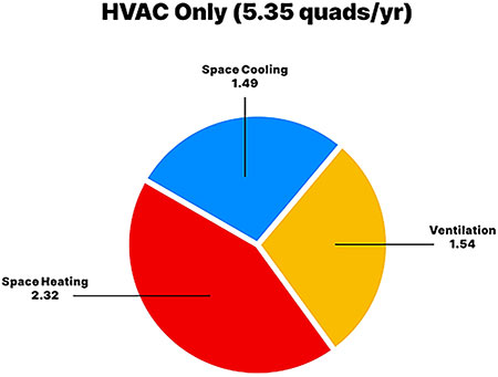
In the 2017 Annual Energy Outlook (AEO), the U.S. Energy Information Administration (EIA) reported that the U.S. commercial building sector consumed roughly 17.83 quadrillion Btu (quads) of primary energy. Of that, HVAC systems consumed 5.35 quads, which was 30% of the total commercial building energy consumption. Nearly a third of that was allocated for cooling.1 (Image 1)
Cooling systems as a whole consume ≥1.49 quads per year. Proportional amounts of energy usage are based on both efficiency and the total number of units in use, so the fact that a piece of equipment tops the list of energy use might reflect more on its popularity than its efficiency:2
- rooftop units (0.74)
- chillers (0.44)
- central split system AC (0.19)
- room AC (0.09)
- gas-fired systems (0.02)
- ground source heat pump (<0.01)
Changing out equipment for more energy-efficient models is always expensive and should be based on a cost-benefit analysis. However, no matter how efficiently a single retrofit is, lowering energy costs can be directly linked to poor ∆T. Inadequate ∆T results in:
- excessive chilled water pumping requirements to deliver the required cooling energy using a lower temperature differential
- reduction in chiller operating capacity
- more chillers running at part load, hindering efficiency
- higher energy requirements at the chillers due to running additional machines outside of their most efficient operating range (at low loads and high flow rates)
- increases in energy consumption for the chilled water pumps
- additional cooling towers and condenser water pumps
- higher condenser water pump and cooling tower energy requirements to support the additional chillers
- excessive equipment wear and reduced life cycles due to higher run times
Flow Rates, System Loads & Lowering ∆T
Typically, chilled water systems retain a reasonable ∆T at high loads up to 12 F (6.7 C). However, at lower loads, the ∆T can fall to <2 F (<1.1 C) resulting in a situation where only a single machine should be operating, but instead, three or four chillers are running to handle the higher flow rates. Over the course of a year, the average ∆T might only be 5.3 F.
Higher flow rates spread across multiple chillers at low system loads means each chiller is operating near the bottom end of its load range, severely depleting system efficiency. Moreover, every time a new chiller is started, the condenser water pump and cooling tower fan(s) might need to operate as well. This increases energy consumption considerably.
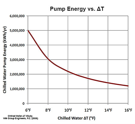
To maximize efficiency, flow rates must be properly managed to correctly sequence the chillers in order to keep each chiller operating near the top of its load range and at higher efficiency levels for as long as possible. Reducing the chilled water flow by improving the ∆T will also have a direct impact on the chilled water pump energy requirements. By maintaining a fixed chilled water ∆T throughout the year, operators should see a reduction in annual pump energy consumption (Image 2).
Water Efficiency & Its Effect on ∆T
Surfactants have been tested for decades to reduce the surface tension of water and improve temperature transfer but not much success had been achieved until the last decade or so. The obstacle was temperature stability within the stream. Relatively recent innovations in nonionic surfactants for both heated and chilled water have provided a new way for facility managers to improve efficiency, lower costs and improve ∆T.
Poured by hand or by metered dosing machine at a designated system intake point, with only a 1% concentration in recirculated water, nonionic surfactants improve temperature transfer from the chilled water to the pipe wall. Doing this accomplishes several energy goals because the system:
- reaches space temperature setpoints faster, decreasing energy load
- lowers fan energy used to retain setpoints
- improves efficiency of all cooling technology in the system
- reduces the number of chiller cycles
- increases ∆T
Across more than 100 case studies on all system types and ages conducted over a decade on a range of facilities, the average reduction in energy and emissions was 15%. Moreover, it was found to be safe to use with both inhibitors and glycols.
Case Study
In the summer of 2019, Allegany College of Maryland added nonionic surfactant to its hydronic system for cooling and experienced a 13.21% reduction in electricity costs and lowered usage by 14.63 kW in a month.
Founded in 1961, Allegany College of Maryland serves students in Allegany County and the surrounding region. The campus is located approximately 150 miles (240 km) from the coast in the foothills of Western Maryland near the town of Cumberland. The average temperature ranges from 77 to 95 F (25 to 35 C) between mid-May to mid-September.
The main campus is comprised of three one-story facilities made from concrete blocks and brick materials common in 1960s construction. Serviced by a 220-ton chiller, the goal of introducing a nonionic surfactant was to reduce the energy costs and emissions for cooling the buildings when classes started in mid-August while the weather was still quite hot.
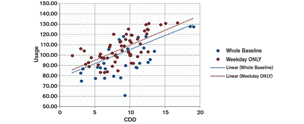
Historical data was only found in electrical bills, which includes non-HVAC consumption, so electrical submetering was installed on the chiller in June 2019 and run to mid-September to establish a baseline. The system was run for three months to model the preinstall consumption versus cooling degree days (CDD) collected from Greater Cumberland Regional Airport at a baseload of 65 F (Image 3).
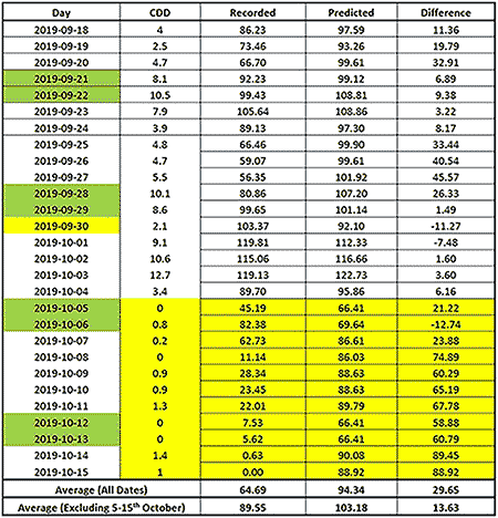
During the analysis, a clear increase during the latter part of summer was detected. This was likely due to the increased usage of the facility as the school year started again. Analysts decided to use the mid-August to mid-September data as the main baseline and the mid-September to mid-October data for analysis (Image 4).
A clear change in system performance was observed during and after the nonionic surfactant was installed. The average power can be converted to consumption to calculate financial savings: energy consumption (kWh) = power (kW) x time (h).
The observed 327.12 kW of electricity has the carbon dioxide equivalent (CO2e) of 231 kg, the same volume of emissions released by a car driving 566 miles. Over a cooling season, the expected greenhouse gas (GHG) reduction is 42.1 metric tons—or the emissions released by nine passenger vehicles traveling over 102,500 miles.
Each day, operators observed an energy saving of 327.12 kW, totaling 5,561.04 kW/h over 17 days. Paying $0.084/kWh, the college experienced financial savings of $467.12. The cooling period is estimated to be six months of the year (circa 182 days). The expected savings is 59,535 kWh or $5,000 per annum with a return on investment (ROI) of two and a half years.
Minimizing Costs by Improving ∆T
No matter how expensive high-efficiency equipment is, the conversation is not “equipment versus nonionic surfactants” but how to maximize a system’s function and reduce costs. By closely monitoring the system, adjusting some operational aspects and improving the efficiency of water, systems of any age benefit.
References
EIA. Annual Energy Outlook 2017. Table: Commercial Sector Key Indicators and Consumption. Reference Case. Aug 2017. eia.gov/outlooks/aeo/data/browser/#/?id=5-AEO2017&cases=ref2017&sourcekey=0
BTO. 2017. Scout Baseline Energy Calculator. Accessed Feb. 2021. trynthink.github.io/scout/calculator.html
WM Group Engineers, “Chilled Water Delta T Study”. Nov. 2008. wmgroupeng.com/sites/wmgroupeng.com/files/CHW%20Delta%20T%20Studynov2008.pdf