University of Florida engineering students benefit from modern modeling technology, 3-D printing and hands-on testing.
Simerics
09/23/2016
A core objective of the undergraduate course Thermo-Fluids Design and Lab in the Department of Mechanical & Aerospace Engineering at the University of Florida (UF) is for students to use a hands-on approach to learn the fundamentals of the fluid mechanics of pumps. In the past, students have used traditional techniques such as Euler’s Turbomachine Equation and velocity triangles to predict pump performance, but these techniques can be inadequate. As a result, UF has begun to explore modern computational fluid dynamics (CFD) to improve these predictions and provide a fundamental understanding of these important concepts.
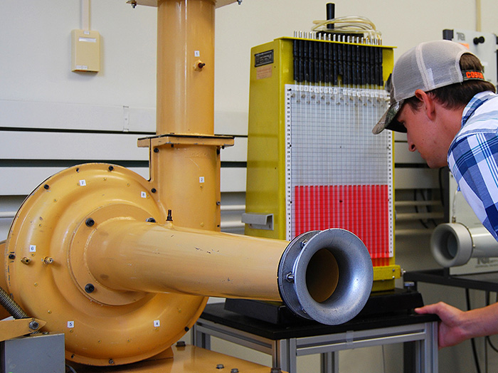 Image 1. Blower housing in test (Images and graphics courtesy of Simerics)
Traditional Techniques
The process begins with the application of Euler’s Turbomachine Equation to determine the blade angles for the impeller. Next, students add the blades to a template of the impeller hub provided by the instructor in a 3-D computer-aided design (CAD) program1 as shown in Figure 1.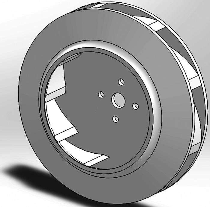 Figure 1. Solidworks drawing of an impeller rig
 Designing Using CFD
Once an initial design is created, the students begin the process of numerically analyzing the impeller’s performance. Numerical CFD simulations are used to test different blade shapes by generating curves of the head rise versus the flow rates and comparing the predictions with the desired performance. Each of the design iterations involves a detailed process. First, the students create a CFD mesh to precisely conform to the geometry provided by the CAD. Then, they implement appropriate boundary and operating conditions. Finally, they select specific numerical parameters to perform virtual tests.Fluid Volume Mesh
First, the students create a model of the test rig and hub assembly using a NextEngine 3-D HD scanner and the CAD program. They then add their impeller designs in the CAD program and extract the system’s fluid volume, saving it in stereo lithographical (STL) format. The STL format includes the triangulation of the surfaces of the inlet, outlet, volute and impeller. This file is imported into the CFD code and used to create the numerical mesh and boundaries needed for the simulation. A typical mesh size for these simulations is about 3 million cells. This process is automated, requiring less than 10 minutes to generate a mesh that captures details down to the order of microns. Students learn guidelines for generating a mesh that will produce accurate results while optimizing the calculation speed. The students then enter the properties, boundary conditions and operating parameters corresponding to what would be done in a physical test. For the simulations, air is assumed as an ideal gas, and the pressure far from the inlet nozzle is atmospheric, with the exit pressure also atmospheric in accordance with subsonic nozzle flow theory. Turbulence is modeled using the standard K-epsilon model2. The flow is regulated with 10 different smoothly contoured nozzles with cross-sectional areas corresponding to 5, 10, 15, 20, 25, 30, 40, 50 and 70 percent of the fully open flow at the outlet. The system is tested with the nine nozzles plus a shutoff plate (for no flow). The geometries of the nozzles, inlet, volute and outlet are included as part of the numerical model. By specifying the geometry, inlet and exit pressures, and rotational speed of the impeller, the CFD code will predict the corresponding flow rate and the head rise.Numerical Parameters
In addition to the operating conditions, several numerical parameters—such as higher-order schemes and transient versus steady-state analysis—must be considered.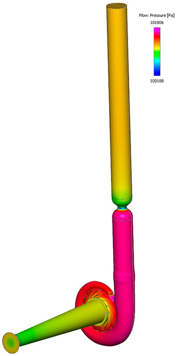 Figure 2. 3-D pressure distribution of the flow field predicted by the simulation
 .jpg) Figure 3. Close-up of the velocity vectors on a plane passing through the fan blades. The goal was to reduce separation in the flow.
Figure 3. Close-up of the velocity vectors on a plane passing through the fan blades. The goal was to reduce separation in the flow. Printing & Testing
Once a prototype design has been selected based on the CFD results, a Stratasys Dimension 1200es or a Fortus 360mc 3-D printer is used to create a physical impeller made of either acrylonitrile butadiene styrene (ABS) plastic or polycarbonate (see Image 2). The printed impeller is subsequently mounted to the fan housing and tested in the UF Undergraduate Fan Performance test bed. The volumetric flow rate through the apparatus is computed by measuring the difference in static pressure in the calibrated inlet nozzle and atmospheric pressure, and computing the velocity based on the Bernoulli equation with an appropriate nozzle coefficient.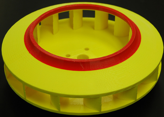 Image 2. Impeller prototype made of ABS plastic, designed and printed by one of the student teams
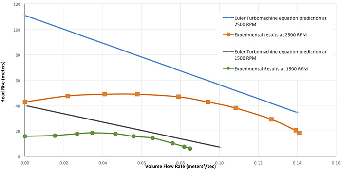 Figure 4. Experimental results at 1,500 and 2,500 rpm. The curve predicted by the Euler Turbomachine Equation is also shown. The experimental curves at each rpm deviate significantly from those predicted by the Euler Equation.
Experimental Results
Students conduct experiments at two different rpms, 1,500 and 2,500, and obtain head rise for flow rates beginning at shutoff conditions. They then increase the outlet flow area until it is 100 percent open. The results are shown in Figure 4. This impeller was designed to have a negative slope throughout its operating range. Using just the Euler Turbomachine Equation, a linear slope of -546 meters per cubic meters per second (m/[m3/s]) is predicted at 2,500 rpm, but the experimental curve deviates significantly from that prediction. The Euler Equation predicts a maximum head of 111 meters at 2,500 rpm at shutoff conditions, while 43 meters was actually obtained. This corresponds to a prediction error of 175 percent. At 1,500 rpm, the Euler Equation predicts a slope of -327 m/(m3/s) and a maximum head of 40 meters at shutoff conditions, while 16 meters at shutoff was obtained in the experiment.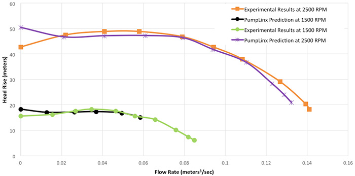 Figure 5. A comparison of the head rise predicted by the CFD tool with the experimental results is shown here. For comparison, one meter of head corresponds to 0.0017 pounds per square inch (psi). Over the range of flow rates from 0.02 m3/s to 0.11 m3/s at 2,500 rpm, the predictions from CFD are essentially identical to the experimental results. Over the entire range of flow rates at 1,500 rpm, the CFD predictions are essentially identical to the experimental results.