Pumping Prescriptions
by Lev Nelik
Pumping Machinery LLC

The objective of this month’s column is to show end users how to hydraulically evaluate their pump systems and determine the power required for the drivers to move the desired flow through the piping/process.

A process designer usually begins a project by determining how much flow must be pumped from point A to point B. The details of the piping, required pumps, coolers, filters and instrumentation are determined based on the flow.

Equations

For example, once the piping is outlined and the system begins to take shape on paper, the designer can calculate pressures at various points within the system. These pressures will be affected by piping length and diameter, plus restrictions such as bends, turns and devices along the flow path.

Once the flow-pressure field is determined, the pump power can be calculated using Equation 1.

In U.S. units, flow is typically measured in gallons per minute (gpm) and head in feet (instead of differential pressure). The k value is equal to 3,960 for BHP to be measured in horsepower (hp) units.

To get an initial “feel” for the motor power and size, the designer may make a rough estimate of efficiency. This can vary greatly depending on the pump type, size and other factors, but an efficiency of 50 percent can be used as a starting point. For example, 3,000 gpm pumped against 200 feet of head would require a 300-hp pump (see Equation 2).

At a later stage, in the design process, this number can be refined based on the more specific curves from the original equipment manufacturer (OEM). From there, the designers can compare multiple bids and make a final selection.

At the initial stage, a rough number (see Equation 2) could suffice if, for example, the designer completes a rough budgetary assessment that shows a certain option is too costly. Often, this approach would be effective, as demonstrated by any typical pump performance curve. Figure 1 shows that efficiency remains relatively constant within a wide flow range.

Pump Performance Curve
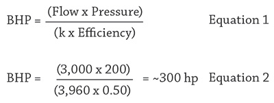
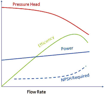
Figure 1. Typical pump performance curve (Graphics courtesy of the author)

OEMs typically do not show pump operation at flows significantly beyond the best efficiency point (BEP), even though the pump could still operate if its curve were extended beyond the maximum flow shown (typically not much beyond 120 percent of the BEP). Pumps typically do not run at the extremes of a curve, but occasionally they do. If the pump is required to operate at flows way past the BEP, a larger pump would be selected, and the operation of a smaller pump at high flow would remain a moot point.

Occasionally, however, this becomes a real issue. An example is a pump required to operate for at least a few minutes in the event of a ruptured discharge pump so operators have time to take the pump offline safely. Nuclear power plant cooling water pumps, for example, must maintain such operation to allow for a slow plant shutdown. Motor trip caused by excessive motor power at high flows can cause problems.

In such rare cases, a better approximation is required. Pump behavior in such unusual conditions can be accurately predicted using Knapp diagrams, which are based on testing in the mid-1930s at the California Institute of Technology and published at The American Society of Mechanical Engineers (ASME) Transactions in November 1937.

These diagrams show pump operation in four quadrants (positive and negative flows, at forward and reverse speeds) for several sample specific speed (Ns) pump designs. These rarely used diagrams are actually very useful for these considerations. Figure 2 shows an example of a Knapp diagram for positive rotation (negative revolutions per minute [rpm] portion omitted for brevity).

Figure 2Figure 2. An example of a Knapp diagram: The red line shows the head-flow (left) relationship at 100 percent rpm and the torque-flow (right) relationship for a 1,800-Ns pump.
Table 1
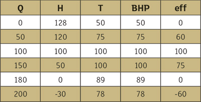
Table 1. The curve from Figure 2 digitized at 100 percent rpm (100 percent efficiency is simply a reflection of the BEP conditions of 100 percent flow, head and power)

The head drops with flow, crossing the flow line (zero head), and continues to drop further (negative head). The torque continually rises (and so would power at a constant speed), similar to the trend in Figure 1, reaching its maximum around 150 percent BEP flow before beginning to decrease. Table 1 shows points on the head-flow curve and torque-flow curve. We can then plot the data in Figure 3.

Figure 3
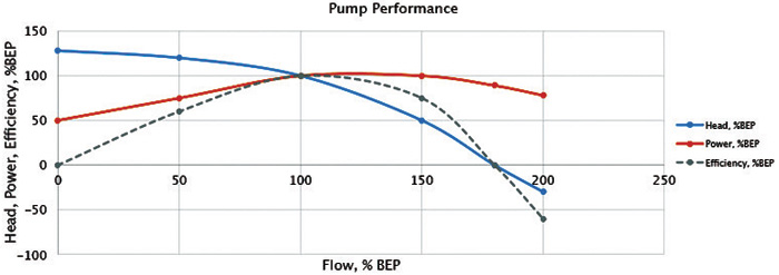
Figure 3. Pump performance curve into the extended flow range

As you can see, a relatively constant efficiency can be assumed for an estimated calculation within the flow range of approximately 50 to 150 percent. Beyond that, efficiency changes dramatically. In fact, at about 180 percent flow (for this Ns example), efficiency hits zero—even negative.

As a side note, at zero efficiency, the pump is still pumping, but power is turned into heat. Once head drops below zero, power is transmitted from the fluid hydraulically to the motor, and the motor becomes a turbine. It takes power from the net, which turns to heat, but the fluid also transmits a component of power to the fluid, heating it. Some power is taken from the total driver power to be used “nonproductively.” The productive part is for flow and pressure. At negative head, fluid receives more heat than the motor delivers to it, with extra heat produced as the pump operates in a highly inefficient turbining mode.

We cannot assume an approximate 50 percent efficiency for a preliminary motor sizing. A Knapp diagram can aid in a more accurate prediction.

To read more Pumping Prescriptions columns, click here.