With continuously increasing energy costs, pump manufacturers must provide energy efficient solutions for fluid transfer. Besides hydraulically optimizing current technology, manufacturers are launching a number of new, highly efficient electrical drives and powerful control systems.
With the focus on optimizing current and new technology, the savings that can be generated with dimensioning a pipeline and specifying the right duty point for a pump in the planning phase are often underestimated.
Pump Power Requirements
A sample calculation will help illustrate the savings potential. A pump's duty point is usually defined by the required flow and the related pressure. The latter is often indicated as head. For turbulent flows of Newtonian fluids, the correlation between pressure loss and head follows a quadratic relationship. Formula 1 applies to a closed pipe system with a static pressure of zero:
H ~ Q2
H = Head
F = Flow
Formula 1. Dependency of head and flow in closed pipe system.
The power requirement of a centrifugal pump is defined in Formula 2.
P1 = Q • H • p • g
ηges
P1 =Power input
p = Density of the medium
g = Gravitational acceleration
ηges = Total efficiency of the unit
Formula 2. Power requirement of a centrifugal pump
Formula 2 implies a flow increase increases the power requirement by a factor of three. In other words, over-sizing the flow by 5 percent results in an increase of the energy demand by more than 15 percent (at constant efficiency). An increased flow of 10 percent raises the energy consumption to 30 percent.
Conversely, the influence of flow on the completion of the flow task depends in a high degree on the application. A heating system, for example, will reach more than 80 percent of its heating power if only half of the flow is provided. In contrast, an undersized pump in the sewage or process technology can cause fatal consequences.
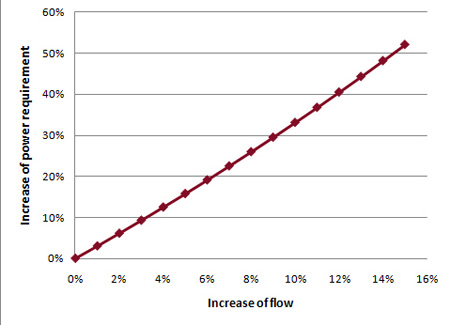
Figure 1. Increase of power requirement follows increase of flow in closed systems.
Planning Tools
Pump manufacturers must support users in the planning phase to guarantee effective pump use. Support can be provided via consultation during the selection process. Various pump manufacturers also offer planning tools in the form of software, particularly web based applications. While complex pipe systems require extensive calculations, applications for unbranched pipes are also available. Numerous pump manufacturers are offering free access to calculation software in combination with a pump selection program.
Web-based software in particular offers a centralized updating process directly on the server and avoids the need for installations on local PCs. In web-based software, the required flow rate has to be determined to size the pipeline and calculate the pressure loss in the second step.
Flow Rate Determination
Each centrifugal pump application has a different calculation for required flow rate. For heating pumps, for example, the required flow results from the heat requirement calculation, but the flow rate in industrial applications depends on the particular transport task and the process parameters. In many applications, international engineering standards are available (which are typically integrated in pipe calculation software programs).
Domestic Wastewater
According to EN 12056, the flow rate for domestic wastewater resulting from drainage can be calculated by adding the run-off coefficients of several sanitary fittings, depending on the building type (see Formula 3).
Qww = K · √ΣDU
Qww = Wastewater drainage
K = Drainage figure according to type of building
DU = Outflow value of sanitary fittings
Formula 3. Calculation of wastewater drainage according to EN 12056
Pipe calculation software programs integrate this formula and the necessary coefficients (see Figure 2).
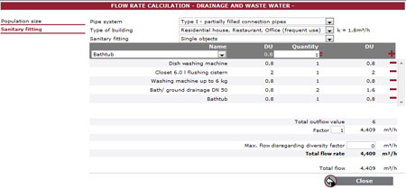
Figure 2. Calculation of flow rate for domestic drainage water according to DIN EN 12056
Alternatively, the flow rate can be determined by the number of inhabitants of a settlement area and the specific peak flow.
Storm Water
For planning and implementation of drainage systems, an updated version of DIN 1986-100, which has to be applied with EN 12056, was released in May 2008. The objective is to size the drainage system so that it offers sufficient protection against flooding. The rain water outflow for a storm water area is calculated depending on the calculated storm water run-off, which is determined statistically (see Formula 4).
Q = r(D,T) • C • A
r(D,T) = Calculation storm water run-off
C = Flow coefficient
A = Effective storm water area
Formula 4. Determination of the rain water outflow according to EN 12056/DIN 1986
Pipe calculation software should contain the statistical values for the calculation as well as for the emergency drainage. Optionally, plot or roof areas for areas below the level of backed-up water can be calculated according to DIN 1986, 14.7.
Drinking Water
To determine the flow rate for drinking water plants, DIN 1988 specifies water sampling points and building types (see Figure 3).
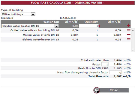
Figure 3. Flow rate determination for the drinking water supply according to DIN 1988
Friction Loss Calculation
If the required flow rate is known, a pipeline can be sized, and the friction loss can be calculated. In many software programs, the system can be divided in several sections and multiple pumps operating in parallel can be considered.
For the friction loss in a straight pipe, Formula 5 applies.
pv = U • L • p • v2 • λ
4A Di
pv = Friction loss
A = Passed cross section area
U = Circumfrence related to A
L = Pipe length
p = Density of fluid
v = Average flow velocity
λ = Friction factor
Di = Inner diameter of the pipeline.
Formula 5. Friction loss in straight pipes
The friction loss in straight pipes depends on the pipe friction coefficient, the cross section, the pipe length and the middle flow velocity. Subject to the Reynolds figure, the pipe friction coefficient λ follows different principles depending on whether it is a laminar or turbulent flow. The pressure loss of valves and fittings is determined via the loss coefficient.
Many pipe calculation programs offer commonly used formulas like those from Colebrook and Darcy-Weisbach or the empiric method of Hazen-Williams.
Total Head
The Bernoulli equation describes the equality of geodetic, static and dynamic energy. The total head consists of pressure losses and static head. The latter results from the geodetic height difference between suction and discharge fluid level and the static pressure difference. In closed cycles, the static part is zero.
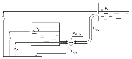
Figure 4. Schematic demonstration of an unbranched pipe system.
Hges = pa - pe + (za - ze) + Hv(Q) + va2 • ve2
p • g 2g
pa - pe = Pressure difference between suction and discharge tank
za - ze = Hges = geodetic height
Hv(Q) = Pressure loss in dependancy flow rate
va , ve = Pipe length
Formula 6. Head of the plant
The term in Formula 6 can be disregarded if the basic cross section on suction-side and discharge-side is sufficient, so the flow velocity is small. Furthermore, the pressure difference is not applicable in open tanks, which simplifies the equation to Formula 7.
Hges = Hgeo + Hv(Q)
Formula 7. Head of the plant with open tanks with a huge cross section
Duty point calculations can be applied directly to pump selection. This is especially interesting for parallel pump operation when different operating modes have to be analyzed.
Pumps & Systems, June 2010